
2D spectra (level 0c).
TECHNICAL NOTICE
RELATIVE INSTRUMENTAL RESPONSE CALCULATION
Objective is to extract relative spectral response of your Lhires III in its 2400 lines/mm configuration, around Ha hydrogene line (dispersion around 0.115A/pixel).
Method described here uses SPiris software for the pre-processing and VisualSpec to calculate this response curve. This last one is calculated by dividing the spectra taken with your Lhires III by a spectra of this same star taken by UVES spectrograph which is attach to one of the VLT 8 meters telescope (Chili).
The selected star in this exemple (Lhires III and a Audine KAF4002ME) is Altair (a Aql). This star is bright which means you should obtain high signal/noise ratio in short exposure time. Also, its spectral profile is very smooth without strong lines. This helps in the method. Altair Ha line is well defined but is also large due to fast rotational speed of the star (Doppler effect).
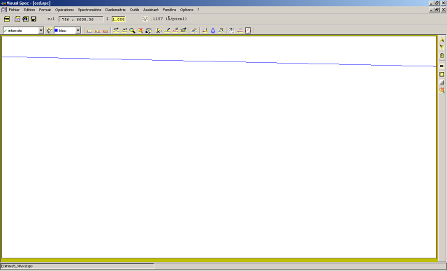
Here is Altair spectre at level "0c", which means pre-processed (bias removal, dark removal, flat division, and all individual frame combined):
2D spectra (level 0c).
This exemple is a combination of 5 individual frames each exposed 120sec. Lhires III is at prime focus of a Celestron 11 (0.28m) telescope. Slit width is 26µm. This spectra was recorded on September 18th, 2006.
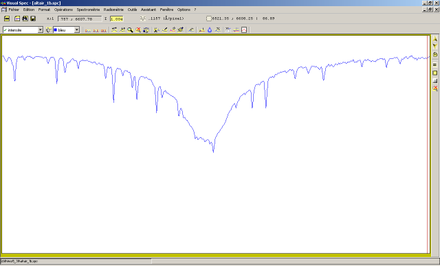
Pre-processing and profile extraction calibrated in wavelength was done in a classical way with the dedicated tool for the "Lhires" on SPiris. Output is a "1b" level spectra (simply extracted and calibrated, no other processing done yet). This profile is then loaded into VisualSpec software:
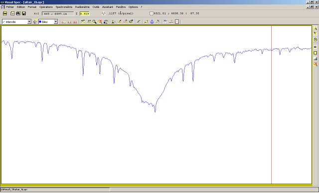
1b level spectra of Altair (VisualSpec)
Step 1 : removing telluric lines
Within menu Options, launch Preferences... Select H2O file with name H2O5.DAT :
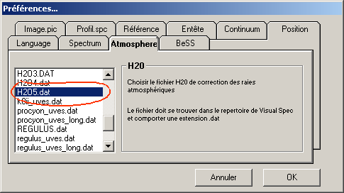
If needed, click here to download this H2O5.dat file and copy it into your VisualSpec install directory (usually c:\program files\vspec).
Validate with OK. (note: the pictures show the french version of VisualSpec but it is similar in the english version).
Then launch H2O correction in the menu Radiometry :
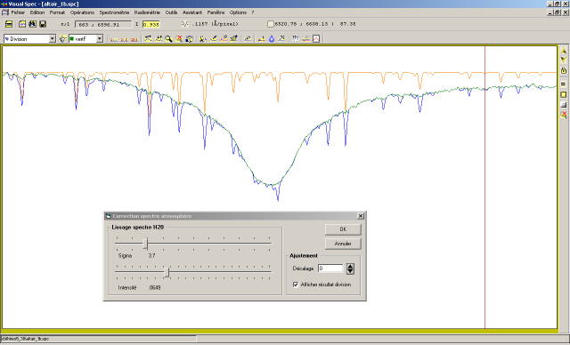
Click on the "display division result" tick to see the result while you adjust cursors to remove as much as you can the telluric lines from water vapor in our atmosphere. With this spectra, best parameters are Sigma=3.7 (this parameter impacts line width) and Intensity=0.0649 (impacts line depth). Here, removal works OK and there is no need to add a "shift" ("décalage" in french on the picture) on the spectra.
Validate your adjustment by clicking OK.
Replace the "intensité" spectra (the main serie of your file) by the result of your division. To do this, click on the "Replace" icone on your toolbar, then click OK in the dialog box:
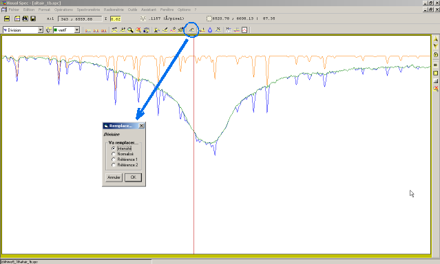
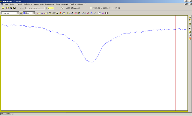
Save the result on the disc. Use the temporary file tmp.spc (for example). Here this spectral profile (equivalent to an Altair spectrum observed with a quasi dry atmosphere):
Step 2 : divide your spectra by a reference spectra.
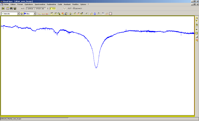
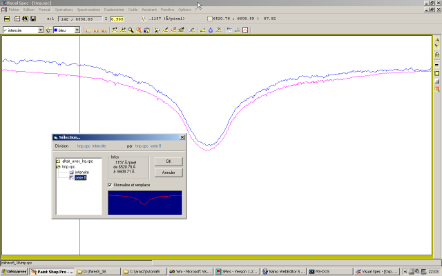
Open both your spectra (tmp.spc) and the one from UVES (altair_uves_ha.spc). This last one is an extract around Ha from the full spectra of Altair taken by UVES. (here a library available of UVES spectra). Click here to download the file altair_uves_ha.spc (1.5MB!). This spectra covers around 6400 to 6700 angstroms:
Copy / Paste this UVES spectra (Edition menu) in your Altair spectra:
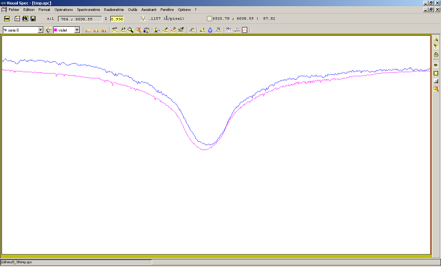
In above picture, UVES spectra is in pink and our spectra in blue. Doppler shift should not surprise as Earth movement projection toward Altair was not the same at observed dates. We can shift or translate the UVES spectra by selecting this spectra and launching the "operations" / "translate" menu:
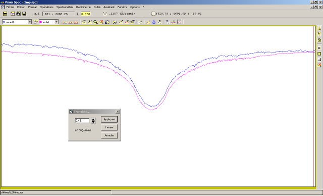
There is here a shifting of 0.45 angstrom. This precision is good enough for our method. Select the blue spectra (our spectra of Altair) and "divide a profile by another" in "operations" menu. Divide by the UVES spectra:
Replace the main serie ("intensité") by the result of this division and save it (file tmp2.spc in our exemple):
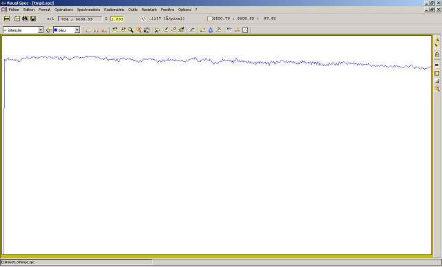
Result of our Altair spectra divided by UVES spectra
Step 3 : extract spectral
response
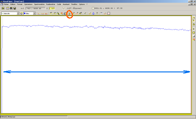
This profile tmp2.spc is almost the spectral response curve but we will remove high frequencies which are noise or remaining of telluric lines....
first, keep only the good portion of the spectra. Crop the spectra to remove invalid values on the left (due to the extraction algorithm in SPiris). Use the cisor tool in your toolbar:
Then run the menu "Radiometry" / "compute continuum" :
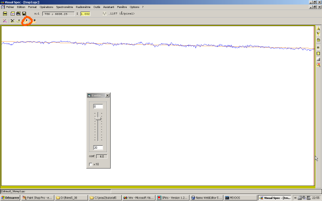
Use the right parameter so you remove the high frequencies only and follow the overall curve profile.
Close the tuning window, replace the main serie ("intensité") with the fitted curve, and save this precious result into a response_curve.spc file:
Final response curve.
This file response will be used to process all spectra taken than night. Take your "1b" level spectra, divide by this response curve, and you get the "1c" leve (instrumental respone corrected spectrum).
This response curve is usually stable enough (for a given configuration) so you do not have to recalculate every night. Specially if flat files are done with the same lamp (ie: same color temperature). Check from time to time that it didn't change by doing this method again.
"1c" level of Altair spectrum, obtained by dividing 1b level with the
response curve.