New features of version 3.80 (November 24, 2002)
Absolute dating of the drift-scan images
Command SCAN carries out a drift-scan acquisition from camera CCD AUDINE (applications are asteroids occultations, mutual phenomena of the Jupiter satellites...). Consult lesson 25 for more details. One of the major problems of this type of activity is to date precisely the event. It is essential to restore for example the circumference of the limb of an asteroid by gathering the observations of several observers distributed on the line of the umbra. It is desirable to reduce measurements with an accuracy of 1/10 of second or better.
After a drift-scan acquisition the files JD.LOG and SHUTTER.LOG are produced by Iris with informations about the date of each CCD lines in Julian day. The information if from the internal CMOS clock of the PC. This one can be synchronized via Internet, or better with sophisticated electronic devices using for example the signals of the GPS system.
New command SCAN_CALIB of version 3.8 offers an alternative to carry out a synchronization in an economic way, rustic, but with a typical absolute precision of 1/10 second. That of which it is necessary use a webcam and of a good watch beating the second on a liquid crystal display. The ideal is to get a clock synchronized on radio signals, which guaranteed the 1/10 of second at least.
Command SCAN_CALIB makes it possible to carry out in fast gust a series of images of the digital watch or a chronograph (about 10 to 15 images a second on a modern PC). A typical sequence of acquisition made from 40 to 50 images. Those are automatically saved on the hard disk. With the analysis, one seeks an image of the sequence which corresponds just to a change of second immediately read on the numercal display. At the same time, with the acquisition of the images in gust, Iris save a text file which for each image contains time in seconds and fractions seconds since the moment of the startup of the PC. There is a very precise instruction in the PC which delivers this information (it forms part of the instruction set of the microprocessor). It is the instruction RDTSC (see for example http://cedar.intel.com/software/idap/media/pdf/rdtscpm1.pdf). The register read by instruction RDTSC changes state with each basic cycle of of the PC clock, i.e. a million times a second on a PC 1 MHz for example. Command CPU of Iris is useful to find the coefficient transforming the contents of the register into seconds (see lesson 25). This time, which one indicates by time-stamp, in addition is encrusted in bottom left part of the webcam saved images.
Moreover, each time that a drift-scan imageis realized with command SCAN, the program produces the file TICK.LOG which is the equivalent of JD.LOG, but containing the value of the time stamp measured to each line of the scan. The TICK.LOG contain the key information to calibrate in absolute the acquisition with reliability.
Here the procedure characteristic to apply at the time of a scan observation.
Step 1
To record the precise value of clock frequency of the PC use the CPU command (this count the number of cycles of the base processor clock during one period given in parameter). Use a long time period for a very good precision, for example 20 minutes (1200 seconds):
CPU 1200
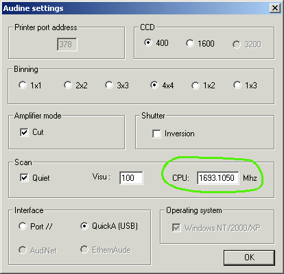
At the end of 20 minutes, Iris return the clock frequency. For example, on my PC Celeron 1.7 Ghz, one found 1693.105 MHz. This value is stable typically with an accuracy of 4.10-6 over one period of several day if the temperature relatively stable. The operation is normally to make once for all for a given computer. One enters the found value of the frequency of the PC in the setup dialog box of Audine camera:
Step 2
A few minutes before the scan film the watch with the webcam during a few seconds by using command SCAN_CALIB. It is necessary to arrange so that the clock is quite enlightened to be able to acquire under good conditions at the maximum rate authorized by the webcam (video Propriety command of menu Webcam). Also privilege a small size image, for example 240x176 with the Philips ToUcam, always to obtain a high speed acquisition. With the 1.7 Ghz PC one thus obtains a frequency of approximately 15 images per second.
For example
SCAN_CALIB START 50
product a sequence of 50 webcam images saved on the disc (into the working directory) under names START1, START2... START50.
Here image START30:

The watch indicates 19h51m13s and PC clock 5571.123 seconds (time stamp).
Now the image START31:
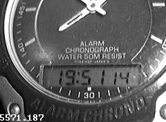
The seconds have just changed on the watch, it is 19h51m14s, PC clock indicates 5571.187 seconds. The time step between this two images is of 5571.187-5571.123 = 0.064 second. This time range corresponds to uncertainty on the evaluation of absolute time, if we consider the perfectly on date.
One will retain that the civil time C1=19h51m14s corresponds to PC time T1=5571.187 seconds.
Step 3
Acquire the scan itself on the object which will be occulted. For example
SCAN 150 350 0.1 2000
The period of acquisition of the lines is here 0,1 second. There are 2000 acquired lines (either a total time of 200 seconds observation). One uses the CCD area between column 150 and column 350..
The text files JD.LOG and TICK.LOG are saved automatically on the disc at the end of the scan. They will be analyzed later.
Step 4
By safety measure, to just remake a sequence images of watch with the webcam after the scan observation:
SCAN_CALIB END 50
Here END18 image:

and here the END19 image, which shows the one second jump
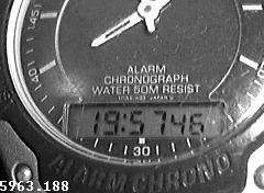
Civil time is C2=19h57m46s whereas the PC tilme is T2=5963.188 seconds.
By way of control let us make the difference of civil time:
C2 - C1 = 19h57m46s - 19h51m14s = 392 seconds
and the difference of PC time
T2 - T1 = 5963.188 - 5571.187 = 392.001 seconds.
The differences in civil time and PC are in coherence. All it passed well between the two the synchronization of the clock time-stamp!
Step 5
Let us carry out the analysis of the drift-scan image. For example try to determine at what time the line number 821 was obtained. Here an extract of file TICK.LOG:
816 5820.050
817 5820.150
818 5820.250
819
5820.350
820 5820.450
821 5820.550
822 5820.650
823 5820.750
824
5820.850
825 5820.950
826 5821.050
Line 821 was acquired at PC time T=5820.550 seconds. Let us make the difference with the first time of reference obtained (T1):
T - T1 = 5820.550 - 5571.187 = 249.363 seconds
So the absolute civil time for the moment of acquisition of line 821 is
C = 19h51m14s + (T - T1) = 19h51m14s + 249.363 = 19h55m23.36s ± 0,07s
(by making the assumption that the watch is perfectly at the date)
Now examine part of file JD.LOG:
816 2452583.330128924
817
2452583.330130081
818 2452583.330131239
819 2452583.330132396
820
2452583.330133554
821 2452583.330134711
822 2452583.330135868
823
2452583.330137026
824 2452583.330138183
825 2452583.330139340
826
2452583.330140498
The moment of acquisition found for line 821 by using CMOS clock of the PC is in Julian day 2452583.3301347, i.e. November 4 2002 at 19h55m23.64s (JD2DATE command under Iris). CMOS clock of the PC is in advance of 19h55m23.64s - 19h55m23.36s = 0.28 second compared to the clock of the watch. But it is the result obtained with the watch which must be taken into account for the analysis of scan.
Support of the QuickAudine interface
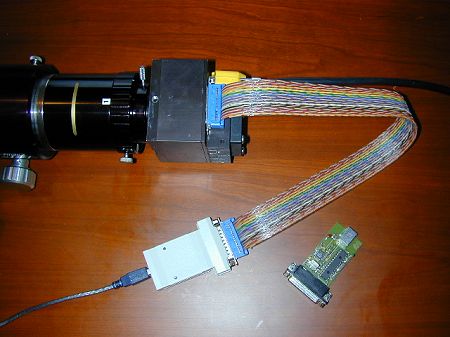
QuickAudine is an USB interface for the Audine camera. In one side it is connects to the camera with a flat cable, which can be very short. On the over side it is connects to the computer via the USB cable. From the characteristic of the USB, the QuickAudine interface is autonomous electrically and simple of use. It allows also a faster reading compared to the parallel port, used traditionally until now.
To use QuickAudine select the QuickA option in the setting dialog box of Audine CCD camera:
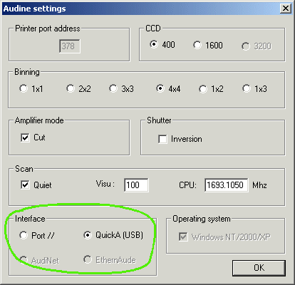
To acquire an image use the ACQ command since the console. The scan acquisition mode is supported for the moment only by the parallel port. For functions more advanced it is necessary to use the Pisco software for example.
For more information on interface USB QuickAudine and its implementation click here and to also consult the site of Thierry Maciaszek.
New commands
ANIM_PLOT [ DATA ] [ OUTPUT ] [ DIM X ] [
DIM Y ] [ YMIN ] [ YMAX ] [ TITLE ] [ NUMBER]
Save
a series of graphics images calculated with the data present in
sequences of file of generic name [ DATE ] (the extension of the file is
.DAT). These data files are text type and contain two columns (axes X and Y
respectively). They are produced for example with command DATA_ANIM. Graphics are saved
in
the form of images of generic names [OUTPUT ] and of size in pixel [DIM X]x[DIM Y]. The
range along the Y-axis is defined with the parameters
[ YMIN ] and [ YMAX ]. The number of data files in the sequence is indicated in
the parameter [NUMBER]. The parameter [TITLE] is a character string which
will be displayed on the top of each graphics. The white character is the
symbol " _ ". Example:
ANIM_PLOT SPECT GRAPH 300 400 800 20000 It_is_a_spectrum 23
See also command PLOT2 which displays only one graph in a similar way and which makes it possible to test ANIM_PLOT. ANIM_PLOT is often exploited in partnership with command DATA_ANIM for the dynamic study of the spectra. An example is here.
BMP2PIC [ INPUT ] [OUTPUT] [NUMBER]
Convert of a sequence 8-bits
BMP 8 images in a sequence of FITS ou PIC images.
PIC_ANIM [INPUT] [OUTPUT]
Function very close to DATA_ANIM. The latter calculates
interpolations starting from data curves, in particular of spectra (click here for an
example). PIC_ANIM
applies to 2-D images to improve fluidity of the animation of a sequences. For
that of the intermediate images are calculated by simple linear interpolation
starting from the acquired images.
The parameter [INPUT] indicate the name of a text file which respectively contains on two columns the name of the acquired images and date of acquisition of these images (or all other identifying function of time, as for example an index value which goes into increasing).
The parameter [OUTPUT] indicate the name of a text filwhich respectively contains on two columns the name of the interpolated images and dates for which the interpolation is calculated (or an identifier function of time, in conformity with that used in the input file).
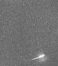
Here an example of application on the trace of a bright Leonid meteor. The observation was carried out by Franck Vaissière by using a modified webcam Vesta Pro long exposure on November 19 2002. Optics is the origin objective of the webcam. Acquisition was made with the sequence mode of Iris. Here 3 images extracted from a sequence of the event:
Suppose 5 images to be interpolated with the names MET1, MET2, MET3, MET4 and MET5. We create in the working directory a text file of name IN.LST containing (use a text editor for that):
met1 1
met2 2
met3 3
met4 4
met5
5
We create the output file OUT.LST:
r1 1.00
r2 1.25
r3 1.50
r4
1.75
r5 2.00
r6 2.25
r7 2.5
r8 2.75
r9 3.00
r10 3.25
r11
3.50
r12 3.75
r13 4.00
r14 4.25
r15 4.50
r16 4.75
r17
5.00
r18 4.50
r19 4.75
r20 5.00
r21 4.50
r16 4.75
r17
5.00
The images R1 and R5 for example will be identical to images MET1 and MET2 (correspondence of the dates). But moreover, between the two images observed, command PIC_ANIM will generate the intermediate images R2, R3 and R4, and so on for the whole of the sequence.
Note: file OUT.LST can be creates automatically with the assistance of command GEN_OUT, which is quite practical for long sequences. In the example one will make:
GEN_OUT OUT R 1 5 0.25
After having saved the file IN.LST and OUT.LST, we produce the interpolated sequence:
PIC_ANIM IN OUT
The sequence R1... R17 synthesized can be visualized with the Animation... command from Visualisation menu. You can also save the sequence in the form of BMP images for produce an animated GIF or a AVI film for example with the assistance of an adequate software:
PIC2BMP R RR 17
You have now on the disc a sequence RR1.BMP..., RR17.BMP.
Here the animated sequence of 27 images of the object which shows the trail well distorted by high altitude differential winds velocity:
Click
on the image to see an enlarged version(750 Kb)
PIC2BMP [INPUT] [OUTPUT] [NUMBER]
Convert of a sequence of FITS
or PIC images to
a sequence of 8-bits BMP images.
PLOT2 [DATA] [DIM X] [DIM Y] [YMIN] [YMAX] [TITLE]
Even function that ANIM_PLOT but applying to only one
data file [DATA].
PREGISTER2 [ ENTERED ] [ LEFT ] [ SIZE ] [ A ]
NUMBER
Even function that PREGISTER for the registration of the
planetary images by the technique of the intercorellation in the Fourier domain. PREGISTER relative make
registration of each image of the
sequence to the first image of this sequence. PREGISTER2 on the other hand
calculates the intercorellation of the image of row N relative with the image of row
N-1. This is of an
interest when the detail which is used to center the images changes of form notably
(a solar protuberance for example).
SCAN_CALIB [NAME] [NUMBER]
Method of synchronization of PC
time. See
the explanation in top of this page.
SMILE [Y0] [RADIUS]
Change the curve of the spectral lines to compensate an
distortion optical defect of smile type, a
traditional problem in spectrograph. The parameter [RADIUS] is the radius of
curvature of the spectral lines. [Y0] is the vertical coordinates corresponding to the vertex
of the curve. For example, here a solar
spectrum in the area of magnesium doublet presenting a significant smile:
The result of the command (radius of -7000 pixels find by successive try):
SMILE 250 -7000
is:

At present, the spectrum can be binned (command L_ADD for example) to extract the spectral profile without risk of loss of spectral resolution. For technical details about the acquisition of this spectrum, click here.
TILT [ X0 ] [ALPHA]
Rectify a spectrum whose axis of dispersion forms an angle [ALPHA] compared to the horizontal axis of CCD
sensor. Calculation is done by
vertically shifting each column of the adequate fraction of pixel. The pivot of
rotation is located at the horizontal coordinate [ X0 ] counted in pixels. The
angle is in degrees and can be signed.
Consider this example of solar spectrum in the area of the triplet of magnesium:
The slope of the dispersion axis appears by the orientation of the transversalium (lines horizontal produced by the irregularities of the input slit of the spectrograph). The tilt is 0.75° (determined by successive tests):
TILT 300 -0.75
Here the result:
|
|
