New features of version 5.32
Version 5.32 - May 6, 2006
Support of the Canon EOS 30D RAW format. Global support of DSRL RAW is improved. The See Exif... command of Digital photo is now compatible with all types of RAW files (the function return primary parameters of the acquisition).
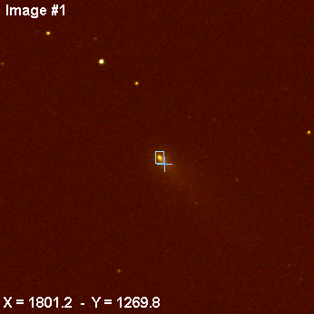
During decoding phase of a RAW file, the date of the generated PIC file (or FITS file) is now conform to the Exif date. The time information propagation of images header is also better along the processing stages. It is an important improvement for process some type of images sequence. Here a typical application. The example below concern an observation of the comet 73P/Schwassmann-Wachmann the 26 April 2006 (fragment C). Canon lens EF 400 mm @ f/5.6 + Canon EOS 350D (with a Baader IR cutoff filter). 20 images of the mobile comet are taken. The elementary exposure is 120 seconds at ISO400. Suburban conditions.
First, construct master images: OFFSET, DARK, FLAT and eventually, a cosmetic default correction file. Click here for details.
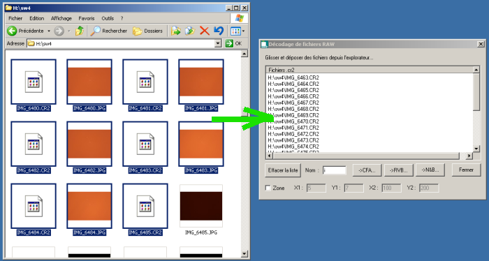
Select the 20 RAW images by helping you of the tool Raw decoding... of Digital photo menu:
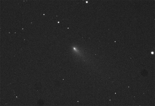
Crop
of a the first RAW image of 73P/Schwassmann-Wachmann (C) comet sequence.
Note the CFA structure and some
dust.
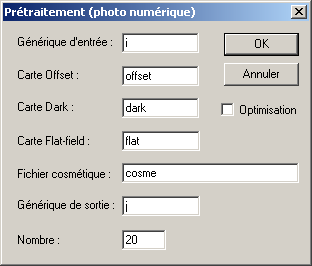
Carry out a traditional preprocessing (Preprocessing... command of Digital photo menu):
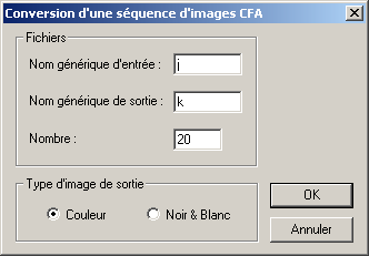
Convert RAW sequence to a RGB sequence (Digital photo menu):
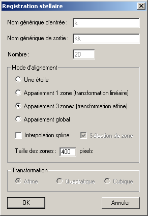
Align the sequence on the field stars (Stellar registration... command of Processing menu):
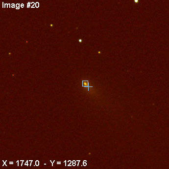
Measure the coordinates of the comet nucleus in the first image and the latest image (use the mouse pointer or, for a more precise result, the PSF command of contextual menu):
|
|
|
Compute the comet displacement in pixel during the acquisition sequence:
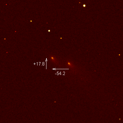
Evaluate the movement in pixels per hour along the x-axis and the y-axis. The elapsed time between the first and the latest is here 0.0345 days, i.e. 0.828 hours (to know acquisition date of an image, load the image and run the command INFO). So we have dx = -54.2/0.828 = -65.4 pixels/hour and dy = 17.8/0.828 = +21.5 pixels/hour.
Process now to a second registration. We take into account the comet movement. Use the command TRANS2. The syntax is:
TRANS2 [INPUT SEQUENCE] [OUTPUT SEQUENCE] [DX pixel/hour] [DY pixel/hour] [NUMBER]
For the example
>TRANS2 KK KKK -65.4 21.5 20
Now stack the registered set of images. The simplest method:
>ADD2 KKK 20
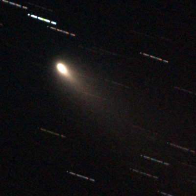
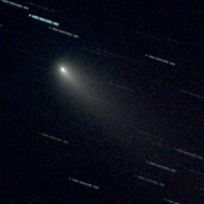
After a DARK command and a minor white balance adjustment; the result:
|
|
|
Left, linear view. Right, logarithmic view
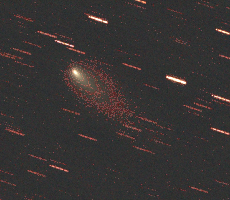
Merge
of a linear view and isophote curves (see Isophotes... command of View
menu).
Note #1: If the comet is bright, it is possible
to align the images with the command REGISTER by selecting the nucleus
with the mouse.
Note #2: For modify of define the acquisition date of a sequence,
use the INIT_DATE command.
For more details about cometary processing, click here.
Version 5.31 - April 17, 2006
NEW COMMANDS
MERGE_HDR [DESCRIPTION FILE] [THREHSOLD]
The MERGE_HDR command is a method for recovering High Dynamic Range images from digital cameras. The algorithm uses multiple images of the scene taken with different exposures and merges the result into a single high dynamic range radiance map of the pixels values.
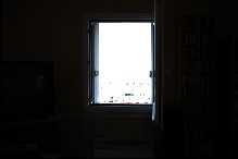
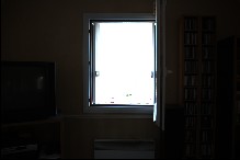
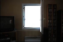
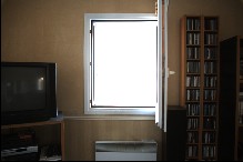
Here is an example. The figure below shows nine shots taken with a Canon 5D Digital SLR with exposure time ranging from 1/500 s to 1/2 s. The image are named T1, T2, ... T9. Clearly, a single view can't recover the entire dynamic of the scene. Each exposure reveals some features that are not visible in the other.
|
|
|
|
|
|
|
|
|
|
|
|
To shoot, a good tripod is useful (or an equatorial mount for sky images), but you can also use the registration function of Iris during a post-processing phase before running MERGE_HDR. Here the colors images are extracted from RAW files (recommended for an accurate work because the linearity response of the DSLR is preserved - it is not necessary the case with JPEG files). The initial dynamic range of the original image is 12-bits (intensity values coded from 0 through 4095).
The first operation is to write a text file with informations about image to process. The file contain two column:
Column #1: the image names of the set of images
Column
#2: the relative exposure time (the absolute value of the exposure time is not
mandatory)
It is the "description file" of the sequence.
For the present demonstration, edit the following text and save filte with the name DESC.LST (for example, only the extension .LST is required) in the working directory:
t1 0.00400
t2 0.00800
t3 0.01600
t4
0.03125
t5 0.06250
t6 0.12500
t7 0.25000
t8 0.50000
t9 1.00000
A very equivalent file can be:
t1 0.00800
t2 0.01600
t3 0.03200
t4
0.05250
t5 0.12500
t6 0.25000
t7 0.50000
t8 1.00000
t9 2.00000
The first parameter of MERGE_HDR command is the name of the description file. The second parameter is an intensity threshold related to the maximum level of the input images. A starting value here can be 4095 in the present example, but do not hesitate to modify the value by trial and error method. The goal is to restitute correctly high level in the merged image. In many situations, select a lower value for the threshold, for example here 2000 (do not be afraid, the intensities level between 2000 and 4095 are conserved in the final result, the threshold act only on the tuning of the internal algorithm).
Run
>MAKE_HDR DESC 2000
At the end of the process time, Iris displays the HDR image. Iris uses 32-bits arithmetic for internal calculation, but in the present version of Iris, the final result is scaled into the 15-bits standard dynamic (0 to 0 32,767 range). The actual dynamic of Iris HDR (V5.31) is only 32767:1 (!). But this can give us some services, as we go. In the present situation, here the new image 15-bits of our scene.
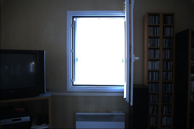
The
15-bits HDR image.
Change the display threshold (up to 32,767 level), and control the high dynamic of the image.
It is recommends that you shoot a minimum of three shots, but preferably between five and seven to cover the entire brightness range of the domestic scene or a deep-sky field. MERGE_HDR can process B&W and true colors images (3 x 16 bits).
REDUCE_HDR1 & REDUCE_HDR2 commands
Syntax:
REDUCE_HDR1 [GAMMA]
REDUCE_HDR2 [GAMMA] [SHARPNESS]
It is not possible to display the huge range of levels of HDR image can contain. You can adjust the image on-screen with a slider, ok, you can see various parts of the dynamic range, but at this point you can't hope to see all of it at once. REDUCE_HDR commands family use methods for rendering the HDR image on your conventional displays. Two methods are presently available.
The first method (REDUCE_HDR1 command) is based on an adaptative logarithmic compression of luminances values for imitating the humain response to light. The parameter GAMMA is a gamma correction to the tone mapped data to compensate non-linearity of displaying devices. Commons values are gamma=1.5, ..., 4.
The second method (REDUCE_HDR2 command) use a gradient method to boost details. The supplementary parameters control the sharp of luminous parts of the image. A typical value is sharpness=1.5.
Example:
>REDUCE_HDR1 4
You can applied on the result some unsharp mask or wavelet to control the sharpness of the image (see Processing menu):
>REDUCE_HDR2 1.8 1.5
If necessary, it is easy to desaturate the image by using the Saturation... dialog box of View menu:
or use the WHITE command for adjust white balance (select a white area with the mouse pointer before):
DESC_HDR [IMAGE NAMES] [DESCRIPTION FILE] [NUMBER]
The DESC_HDR command helps you to define the description file for the MERGE_HDR command if the relative exposure time of the images is unknow or inaccurate. DESC_HDR evaluates the mean relative intensity of a user defined area of the each images. The ratio of the computed intensities is the relative exposure time find in the produced description file.
[IMAGE NAMES] is the generic name of the sequence.
[DESCRIPTION
FILE] is the name of the description file.
[NUMBER] is the number of images
in the sequence.
Before running the command, define a small rectangle with the mouse pointer in an unsatured part of all the set of images (use the most exposed image for identify the unsatured region).
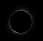
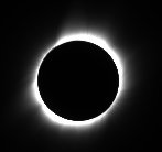
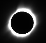
Example. Here a sequence of seven progressive exposures of the 29 March 2006 eclipse (images Valérie Desnoux - Refractor Halley 70/400 mm and Nikon D70 DSLR) :
|
|
|
|
|
|
|
|
First, the Nikon RAW images are converted to PIC files. Second, the offset of the images is removed. It is important to define the true zero of the intensities scale. Use for example a command like:
>SUB2 ECLIPSE OFFSET ECLIPSE 0 7
where ECLIPSE is the generic name of the images to process and OFFSET is an offset master map of the camera.
Then, load the most exposed image and select an unsatured region (but with a significant signal):
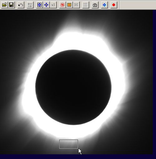
Run the command:
>DESC_HDR ECLIPSE DESC 7
Iris generate the file DESC.LST in the working directory with the content:
eclipse1 0.016032
eclipse2 0.032064
eclipse3
0.066132
eclipse4 0.128257
eclipse5 0.254509
eclipse6 0.517034
eclipse7
1.000000
Now, merge the seven images:
>MERGE_HDR DESC 100
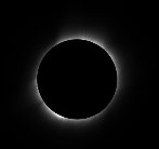
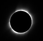
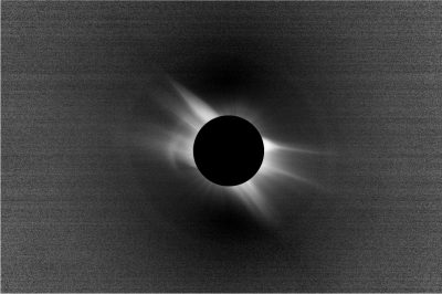
The result is a 15-bits images of the corona:

and now, compress the dynamic:
>REDUCE_HDR1 4
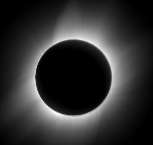
Note the simultaneous visibility of prominances and coronal jets.
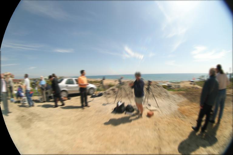
RADIAL BLUR METHOD
RADIAL_BLUR [XC] [YC] [FILTER STRENGTH] [METHOD]
[XC] [YC] are the coordinates of the blur center
[FILTER STRENGTH] is the amount of filter applied.
Typical values are between 0.5 and 20.
[METHOD] if method = 0, spin blur; is method = 1, zoom blur.
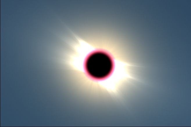
Just
after the 29 April 2006 total eclipse (Turkey).
>RADIAL_BLUR 906 512 18 0
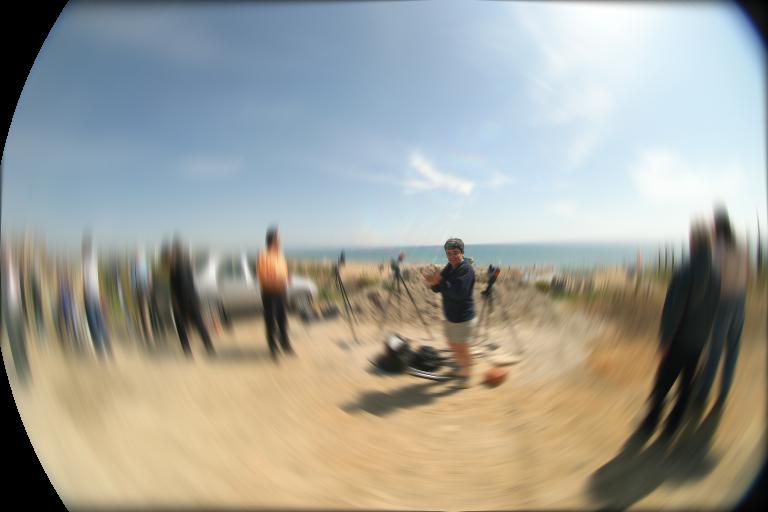
>RADIAL_BLUR 906 512 5 1
RADIAL UNSHARP MASK FILTER - automatic method
ANG_FILTER [XC] [YC] [FILTER STRENGTH]
Simplified and improved version of the initial angular filtering procedure of Iris.
[XC] [YC] are the coordinates of the blur center
[FILTER STRENGTH] is the amount of filter applied. Typical values are between 0.5 and 5.
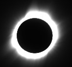
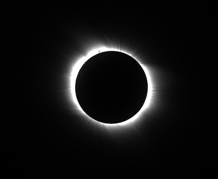
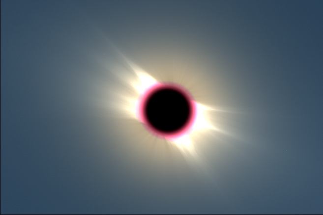
A typical application: enhance and sharp structure of sun corona.
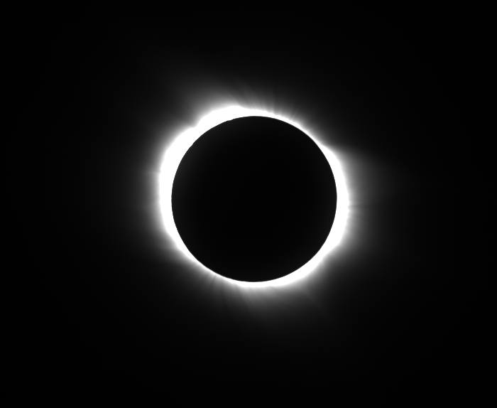
29
March 2006 total solar eclipse. Canon EOS 5D + Canon lens 400 mm f/5.6
Note the coordinates of the disk center (fractional values are possibles). Here XC=2264 and YC=1421. Choose a filter amount of 2.5. Then
>ANG_FILTER 2264 1421 2.5
The result is equivalent to spinned unsharp masking. First, Iris produce a radial blur. Second, Iris subtract the original image and the blurred image. The result is displayed:
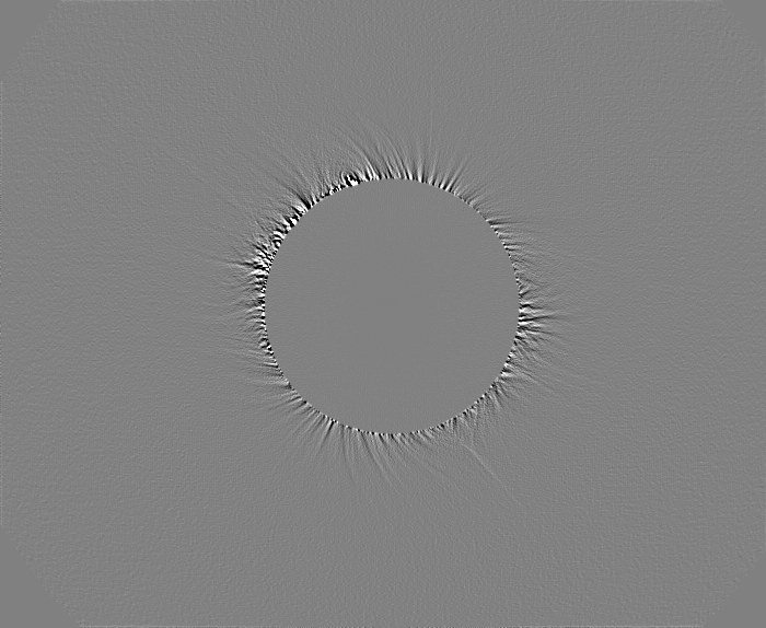
Try some values for the filter strength (trial and error method)
An application is to merge the starting image with the spinned unsharp mask. For this, you can use the new Merge... command of Iris V5.31 (View menu):
In this example, C1 is the original image and C2 is the unsharped image. Iris compute here the image:
(1-0.9) x C1 + 0.9 x C2
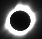
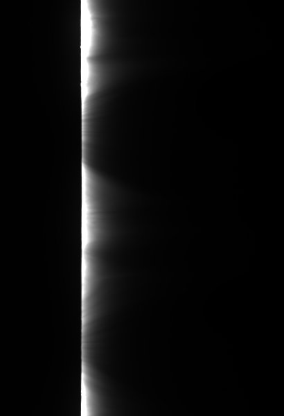
RADIAL UNSHARP MASK FILTER - Manual method
Here, the image to process:
29
April 2006 total solar eclipse. Canon EOS 5D + Canon lens 400 mm f/5.6
Measure the sun disk center position (here at XC=2264, YC=1421) and the apparent sun disk radius in pixels (here R=2065). Note the size of the image (X=4386, Y =2960) and compute the mid-diagonal size of the image: SQR(X2+Y2))/2=SQR(43862+29602)/2=2646. The later is the recommended value of the third parameter of REC2POL and POL2REC commands (but a smallest value is accepted). The first and the second parameters of the commands are (XC, YC) coordinates. The last parameter is the scale of the polar transformation. A suggested value is 0.1 degree / pixel (reduction of interpolation errors).
Evaluate a polar transformation:
>REC2POL 2264 1421 2646 0.1
>SAVE
TMP1
Blur along the vertical axis:
>L_BLUR 6 (a
box blur function)
>SAVE TMP2
or
>L_GAUSS 1.5
(a gaussien blur function)
>SAVE
TMP2

Compute a vertical unsharp mask:
>LOAD TMP1
>SUB TMP2 0
>VISU
100 -100
>SAVE TMP3
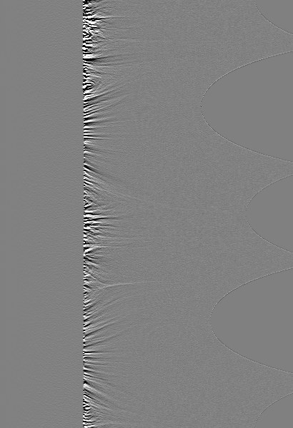
Compute a forward rectangular transform:
>POL2REC 2264 1421 2646 0.1
and restore the initial image size:
>PADDING 4386 2960
Merge to the initial image:
RADIAL_WEIGHT [X] [Y] [RADIUS] [COEFFICIENT] [POWER]
Multiply the intensity I(r) of a given pixel image by a Lorentz function of the form:
where r is the distance relative to a center of coordinate (xc, yc), r0 is an offset radius, coefficient and power are adjustment parameters of the function shape. Normally , power=2.
The parameters x, y, r0, coefficient and power are the successives argument of the RADIAL_WEIGHT command. A typical application is the simulation of a radial density filter during a total eclipse observation. Here some examples:
29
April 2006 total eclipse. Canon EOS 5D & Canon 400 mm f/5.6 L. Stack of
2x2 sec. exposures + 2x1 sec. exposures.
The central region is saturated.
After
command: RADIAL_WEIGHT 2272 1418 220 500 2

After
command: RADIAL_WEIGHT 2272 1418 250 500 2
After
the command: RADIAL_WEIGHT 2272 1418 250 800 2
A
final composite. Images of the photosphere and of a rotational gradient image
of the lower corona are added (see below). The saturated part of the image is
masked (DISK1 command, description
here). Click
here for details about this 2006 eclipse observation.
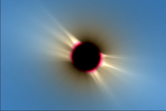
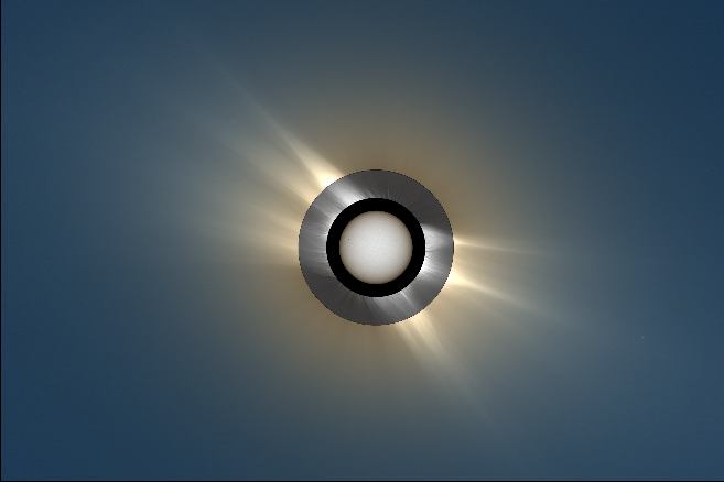
ROTATIONAL GRADIENT FUNCTION AND MERGE DIALOG BOX
Rotational gradient is a good alternative for enhance coronal features (support now true-colors images). The intermediate corona of the image below is enhanced by using the Rotational Gradient function of Processing menu (for 16-bits images only) with the parameters:
Rotational
gradient on an image taken with a cumulative exposure time of 6 seconds (Canon
EOS 5D + Canon de 400 mm @ f/5.6).
Note the central saturated zone.
Below, a composite of the external corona, of the inner corona (rotational gradient filtering), and of a photospheric image :
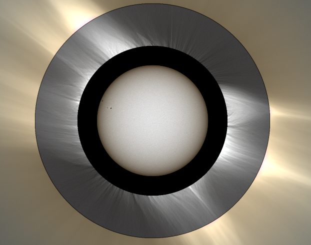
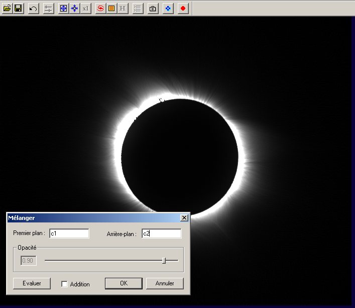
Before insert in the outer coronal image, DISK1 and DISK2 are used for mask undesirable region (click here for a related topics). For the merging you can use a simple ADD command or use the interactive tool Merge... of Visu menu (overlay mode):
Change the slider position for modify the opacity of the front image (T1) relative of a background image (T2):
The computed image is here:
(1 - 0.18) x T1 + 0.18 x T2
If you check the Add button:
the operation is
T1 + 0.18 T2
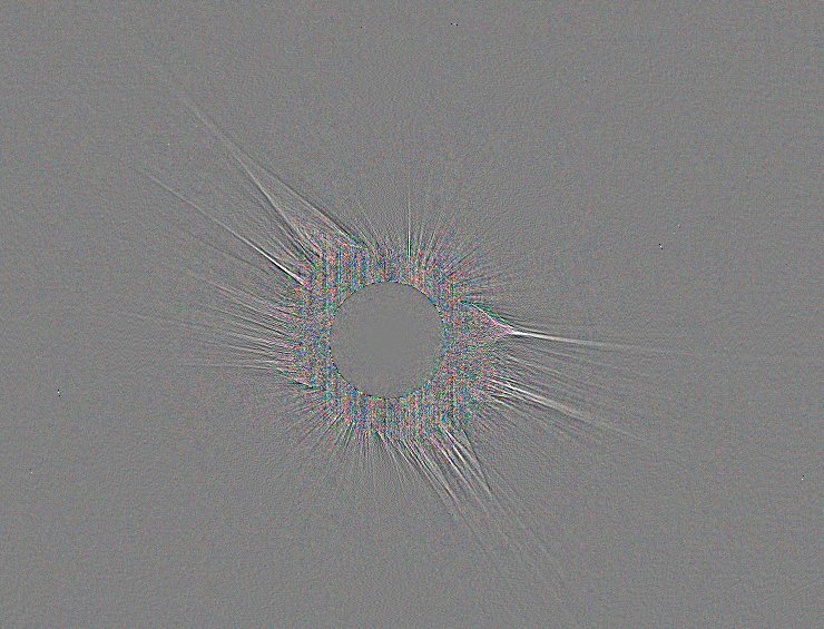
A bug is fixed in the POLAR_CARTO command (display of a vectorial form of a polarization map). Click here for details about the function and here for the March 2006 total solar eclipse application.
Polarization
degree of the sun corona.
|