IRIS TUTORIAL
Comet
image processing
Preprocessing
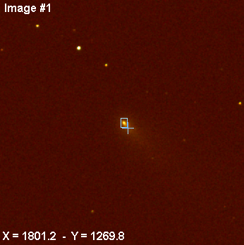
The example below concern an observation of the comet 73P/Schwassmann-Wachmann the 26 April 2006 (fragment C). Canon lens EF 400 mm @ f/5.6 + Canon EOS 350D (with a Baader IR cutoff filter). 20 images of the mobile comet are taken. The elementary exposure is 120 seconds at ISO400. Suburban conditions.
First, construct master images: OFFSET, DARK, FLAT and eventually, a cosmetic default correction file. Click here for details.
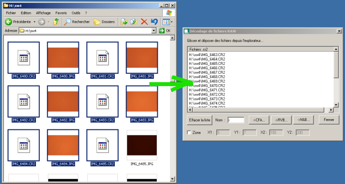
Select the 20 RAW images by helping you of the tool Raw decoding... of Digital photo menu:
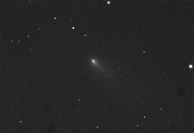
Crop
of a the first RAW image of 73P/Schwassmann-Wachmann (C) comet sequence.
Note the CFA structure and some
dust.
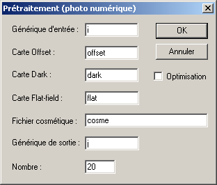
Carry out a traditional preprocessing (Preprocessing... command of Digital photo menu):
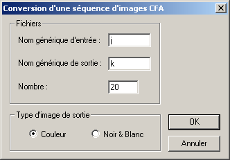
Convert RAW sequence to a RGB sequence (Digital photo menu):
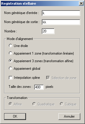
Align the sequence on the field stars (Stellar registration... command of Processing menu):
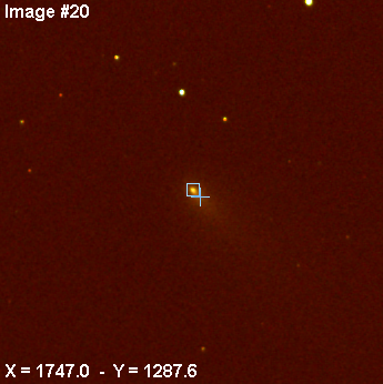
Measure the coordinates of the comet nucleus in the first image and the latest image (use the mouse pointer or, for a more precise result, the PSF command of contextual menu):
|
|
|
Compute the comet displacement in pixel during the acquisition sequence:
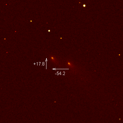
Evaluate the movement in pixels per hour along the x-axis and the y-axis. The elapsed time between the first and the latest is here 0.0345 days, i.e. 0.828 hours (to know acquisition date of an image, load the image and run the command INFO). So we have dx = -54.2/0.828 = -65.4 pixels/hour and dy = 17.8/0.828 = +21.5 pixels/hour.
Process now to a second registration. We take into account the comet movement. Use the command TRANS2. The syntax is:
TRANS2 [INPUT SEQUENCE] [OUTPUT SEQUENCE] [DX pixel/hour] [DY pixel/hour] [NUMBER]
For the example
>TRANS2 KK KKK -65.4 21.5 20
Now stack the registered set of images. The simplest method:
>ADD2 KKK 20
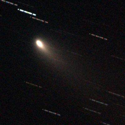
After a DARK command and a minor white balance adjustment; the result:
|
|
|
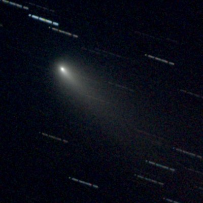
Left, linear view. Right, logarithmic view
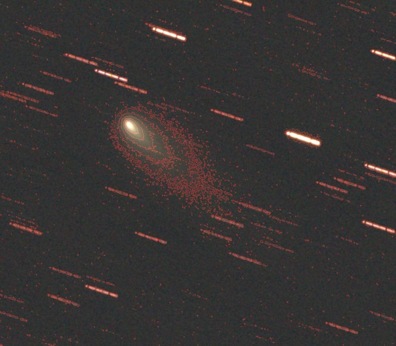
Merge
of a linear view and isophote curves (see Isophotes... command of View
menu).
Note #1: If the comet is bright, it is possible
to align the images with the command REGISTER by selecting the nucleus
with the mouse.
Note #2: For modify of define the acquisition date of a sequence,
use the INIT_DATE command.
Contrast enhancement
Comets are diffuse objects whose details are not very contrasted (jets, plasma tails, etc.). Iris has several tools that allows you to extract these details in a particularly efficient manner. The range of applications is vast: photometry of the nucleus, global photometry, bringing out the rotation of the nucleus, polarization studies, multi-color analysis, etc...
We are going to process a sequence an image of the comet Hyakutake (click here for download HYAKUTA image, size = 110Kb):
>LOAD HYAKUTA
>VISU 1300 300
Standard (linear) view
of the Hyakutake image.
This image clearly shows the large difference in levels that exist between the central region and the rest of the coma (note that the comet occupies the whole image). This makes it difficult to visualize weakly contrasted details. You can try a better visualization (logarithm processing):
>LOAD HYAKUTA
>OFFSET -300
>LOG 10000
>VISU 10000 400
>MODULO 400
>VISU 400 0
Log view of Hyakutake
comet. Note the extension.
Now try to extract the jets that may emanate from the core. First, determine the position of the nucleus. We find the coordinates (171, 164). Then use the rotational gradient, the RGRADIENT command. The syntax is:
RGRADIENT [XC] [YC] [DR] [DALPHA]
Starting from an input image (in memory), RGRADIENT creates two images, with a radial shift ([dr] in pixels) and a rotational shift ([dalpha] in degrees) with respect to the point ([xc], [yc]). Between these two images, the shifts have the same amplitude, but an opposite signs. The two images are then added to create the final image. In polar coordinates (r, a) with respect to the point ([x],[y]), we have:
B'(a,r,da,dr) = 2.B(a,r) - B(a-da, r-dr) - B(a+da, r-dr)
with:
B = the starting image
B' = the resulting image
da = the parameter
[dalpha] of the command
dr = the parameter [dr] of the command
The rotational gradient is used to observe poorly contrasted details in a bright object which exhibits a symmetry of revolution (dust in an elliptical galaxy or jets in the tail of a comet). The gradient removes the object with a symmetry of revolution with respect to ([x], [y]).
>LOAD HYAKUTA
>RGRADIENT 171 164
0 15
>OFFSET 1000
>VISU 1700 600
You can also execute RGRADIENT command from the Processing menu:
Hyakutake image after
RGRADIENT processing. Several jets are clearly revealed by this method.
The gradient produces an image with zero average intensity. The offset is adjusted so that the image can be visualized with positive thresholds. Now, several jets coming out of the nucleus are evident. Be careful when interpreting the results obtained with this technique. Too large a value for [dalpha] can make false details appear, or restore them with an incorrect morphology. On the other hand, too small a rotation angle can keep low contrast structures from being visible.
It is good to experiment with several values of the parameters to have a precise idea of the structures that are revealed. Typical values of [dalpha] go from 2° to 20°. For [dr], the values are from 0 to 2 (negative values are also significant). Finally, note that it is necessary to know the position of the center of the object with precision.
Now, try the angular filtering, i.e. the ANG_FILTER command
ANG_FILTER [XC] [YC] [RADIUS] [SIZE]
The command performs a low-pass filter on rings centered to ([xc],[yc]). The algorithm computes the average of pixels in the ring in sectors of [size] degrees. The size of the computation relative to the center (xc,yc) is a circular area of dimension [radius].
The ANG_FILTER command is generally use to enhance radially structured features in images, such comet or a solar jets visible during a total solar eclipse.
>LOAD HYAKUTA
>ANG_FILTER 171 164 108 31
>SAVE I
>LOAD HYAKUTA
>ANG_FILTER 171 164 108 0
>SUB I 1000
>VISU 1200 900
Result of the angular
processing.
We can also use the mathematical modeling of the coma with the FIT_ELLIPSE command from the Processing menu (for details, click here).
>LOAD HYAKUTA
then:
Here Xmin...Ymax are equal
to zero. In this condition, Iris compute automatically this parameters.
Result of the subtraction
of the model. Note the presence of fine knots in the trail.
See also the wavelet processing of comet images.