
Internal
Data Reduction Methods for eShel Spectra
This page describes the ISIS procedure for reduce spectra taken with eShel spectrograph. This pipeline start with a sequence of 2D raw images (two-dimensionnal images as at the output of detector) and finish with a list of processed spectral profile (one per echelle order).
1. Preprocessing
For each input raw spectra image of the processed object, ISIS substract the electronic offset, the dark current map, divide by the Pixel Response Non Uniformity map (PRNU map). Mathematically:
Preprocessed image = m x (raw image - offset map - k x (dark map)) / (PRNU map) (eq. 1)
The signification of m and k coefficients is given below.
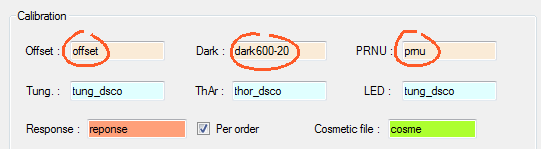
Preprocessing
reference map images.
The offset image value traduct the camera output level for a virtually zero integration time image. The offset image is independ of the integration time and always present into each acquired images.
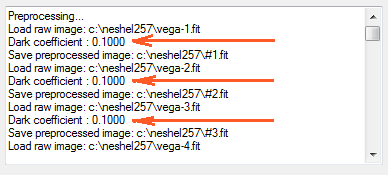
The dark image signature arise from the thermal electrons. The dark signal (or thermal signal) increases with the detector temperature and with the integration time. Dark map is not necessary obtained at the same integration time of the raw input images. For adjust the coherence between dark reference image raw image, ISIS compute the coefficient k, as
k = (raw image integration time) / (integration time used for produce the dark reference map) (eq. 2)
|
|
The PRNU map correct the detector pixel to pixel variation of sensitivy. PRNU frames are obtained by a relative uniform illumination of CCD surface. The processing of PRNU reference map is completed by a low passband spatial filtering for remove slow variation in each individual PRNU frames (unshap masking method) and by a median sum of these individual frames.
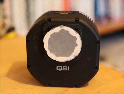
Diffuser
set at the entrance of the camera for the acquisition of PRNU frame.

A
typical PRNU master frame.
ISIS compute the mean of PRNU master, the m-coefficient, for conserve the same typical signal level in the raw input image and in the preprocessed images (see equation 1).
The preprocessing is completed by an optional cosmetic correction if the field "Cosmetic file" is completed:
|
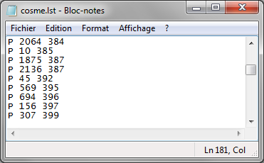
Here, ISIS correct the level of some deviant pixels identified in the ASCII format file "cosme.lst" (by a local mean method, i.e. the deviant pixel is replaced by the median mean level of the 8 neighbors pixels). |

|
Typical cometic file, a list of bad pixels (bad pixels are here identified at coordinates (2064, 384), (10, 385), ... |
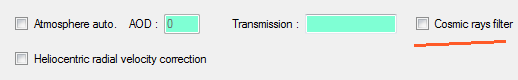
Finaly, a cosmic rays correction can be made (it is an option). Cosmics-rays (high energy particles) often hits the detector surface during integration time. The pixels hit by cosmic rays have high level value and considered as deviant. The cosmic rays correction is actived if you check the option "Cosmic rays filter":
The cosmic ray detection algorithm is based on an iterative threshold method. Warning: it is a time consuming procedure. A Neighbors pixels are used for replace pixels affected by cosmic-ray hits.
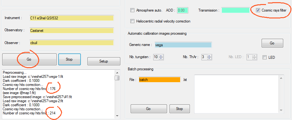
For each
processed images, ISIS return the number of cosmic-rays hits detected
if the option "Cosmic rays filter" is actived.
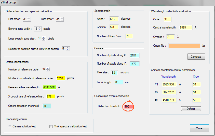
You can adjust the detection sensitivity from the eShel Setup dialog box. A value of 100 for the parameter is often ideal (choose values 50, 150 for test):
For locate the position of detected hits, open the images "@mapxxx.fit". For example:
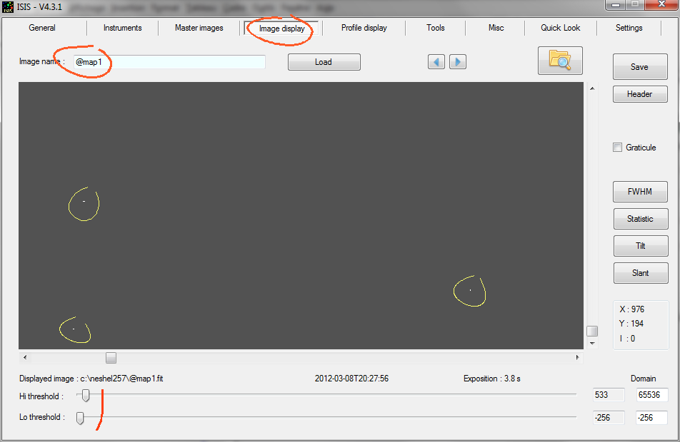
Display the binary image @mapxxx.fit for locate detected cosmic-rays (255, 0 level image).
For the example below, the detection threshold is too low (10), so the number of hits detected is too large (90000!) and not significant (i.e. consequence is false detections):
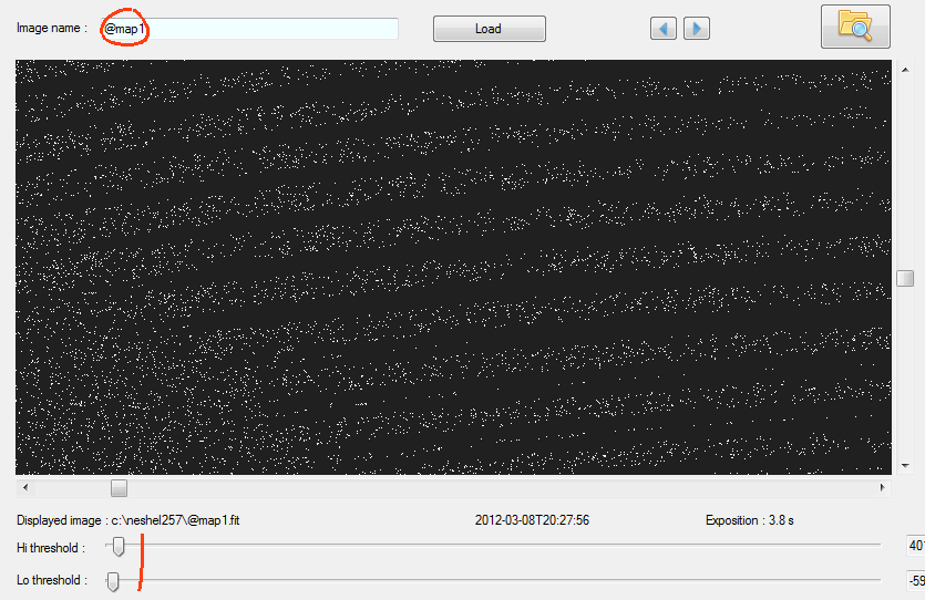
Effect of an incorrect thershold value during cosmic-ray events correction. Many valid pixels are flagged by error.
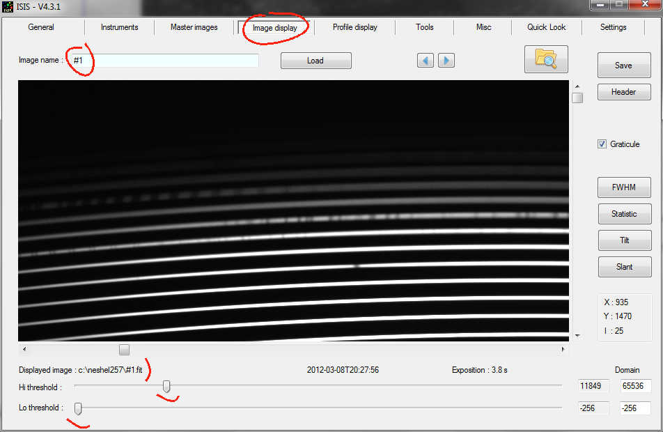
The individual input science processed are saved under the name "#xx.fit", where "xx" is the image index number. Of course, you can display these images for checking, for example:
2.
Detection of vertical position of valid order
Starting from the Y (vertical) measured coordinate of reference order (see example below, order #34 at Y = 1210)
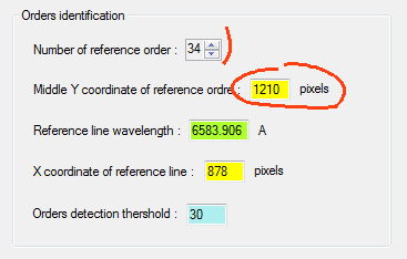
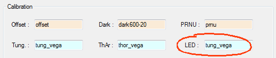
ISIS analyse the given "LED" image for detect significant order relative to the "Orders detection threshold" value (30 in the example), and return the image Y-coordinate of each detected order (at the center of the image):
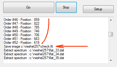
Mid-vertical position of order #46 is Y = 859, mid-vertical position of order #47 is Y = 822, and so on...
At the condition of high signal to noise ratio, the LED image can be replaced by a tungsten lamp spectrum:
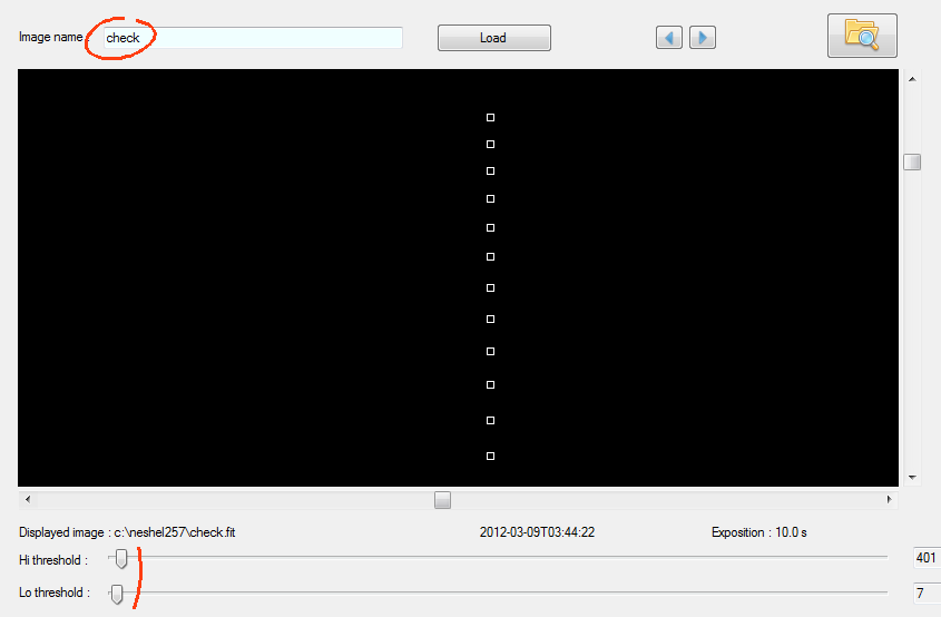
ISIS write a "binary" checking image (level 32000, 0) - named "check.fit" - containing small rectangle at the position of detected orders :
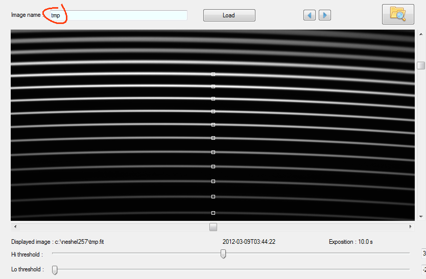
You can make the fusion of check image and "LED" image
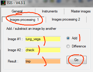
and display the result for checking
3. Orders trace along the wavelength axis
ISIS load in memory the contain of file "del_order.lst":
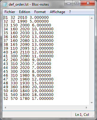
The elements of the file are defined by the user and can be considered as instrumental constant of a given setup.
Colum #1: Correspond
to the order index.
Colum #2 & #3: Define the valid
extension limits of a given order along the horizontal axis of the
image, in pixel coordinates (X1, X2).
Colum #4: The line slant
relative to the dispersion axis in degrees. If the angle is 0°,
the long axis of fiber image on the detector is perpandicular to
the dispersion axis.
For each spectral order find in the "LED" image, ISIS adjust a 4th degree polynom along the individual trace between X1 and X2 coordinates. It is a measure of spectra distorsion banding in the raw 2D images.
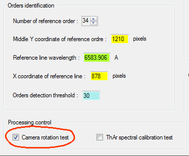
An easy and quick fit quality control method consist to select the option "Camera rotation test" from the eShel setup panel:
Now run the processig...
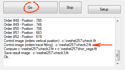
and examine the image check2.fit...
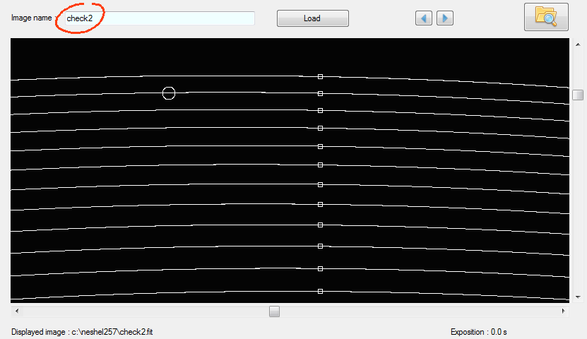
The optical distorsion of spectral orders is now know (a set of polynomial fit equations).
4. Extraction of 2D images of each order
Starting from order indentification, geometrical distorsion correction is made first along the spatial direction (curvature correction of spectral segments), order per order, for the reference tungsten spectrum and for the reference Thorium-Argon spectrum (ThAr). After these geometrical transformations, the dispersion axis is parallel to the X-image axis (the computated parameters are specifics to a given order).
Then the background is substracted (see next section fordescription)
The line inclinaison (slant effect) is corrected by using values given into the file "def_order.lst" (colum #4). IRIS uses spline interpolation for this. After slant correction, the ellipsoidal long axis of monochromatic fiber images (induced by anamorphose effet of spectrograph optic) is now vertical.
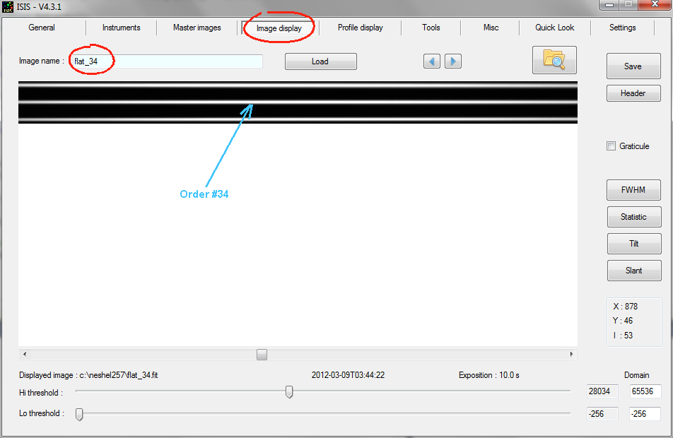
Finally, each segment of spectrum (one for each order) is cropped and saved in individual 2D files named "flat_xx.fit" for tugsten spectrum and "calib_xx.fit" for ThorAr spectrum, where "xx" is the order number :
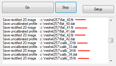
Here an example of spectrum segment for the tungsten lamp (original full 2D master spectrum file name is "tung_vega" in your example):
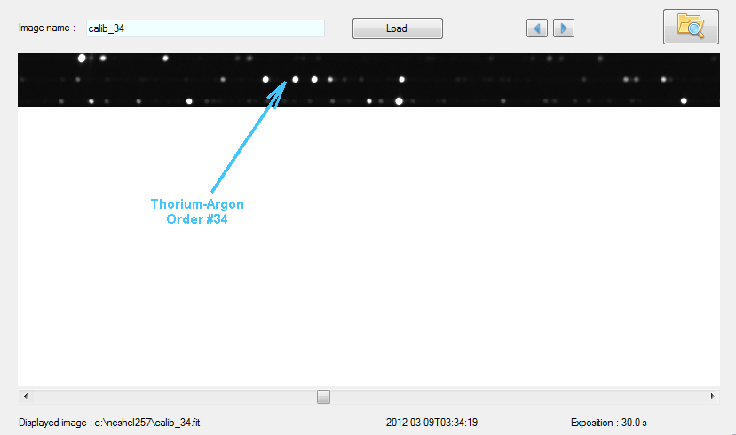
and for the Thorium-Argon lamp (original 2D file name is "thor_vega"):
5. Background evaluation and substraction to reference spectra sub-images
The level of background at the level of a segment spectrum (induced by scattrering light) as a function of wavelength is evaluated along two horizontal lines located in the middle of two consecutive orders. These two lines are drawn in yellow in the next figure:
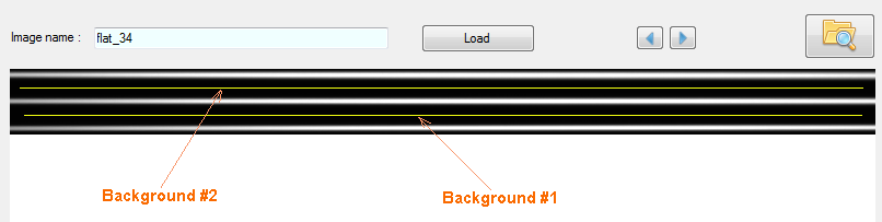
Two distinct polynomial 5-th degree are adjusted along these two lines by using a classical least square fit method. These functions reflect the typical background level under the 2D-spectrum. We calculate the average for the two intensities found by polynomials at the top and bottom of the trace for each point of the spectrum. During polynomial fit, the algorithm excludes any points beyond the level of 1000 ADU up to the mean background value (for avoid large hot spots or cosmic-rays not identified and incorrectly processed before).
The background found by using the two polynomial functions is substracted to the corresponding 2-D spectra segment, colum by colum.
The same operation
is conducted for "flat" and "calib" sequences
of spectra segment.
6. Extraction of profile from reference spectra sub-images
Now the spectral profile of each order image is optimally extracted by using a method similar descripbed by J. G. Robertson (PASP 98, 1220-1231, November 1986). The signal along column is pondered before summation in function of vertical distribution in the 2D spectrum trace (across dispersion axis). The method optimize the signal to noise ratio for faint spectra.
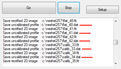
The raw spectral profile are saved under ASCII file sequence named "flat_xx.dat" and "calib_xx.dat":
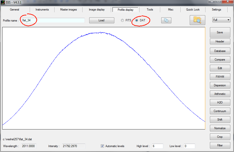
Signal distribution along spectral tungsten lamp order #34 (for example).
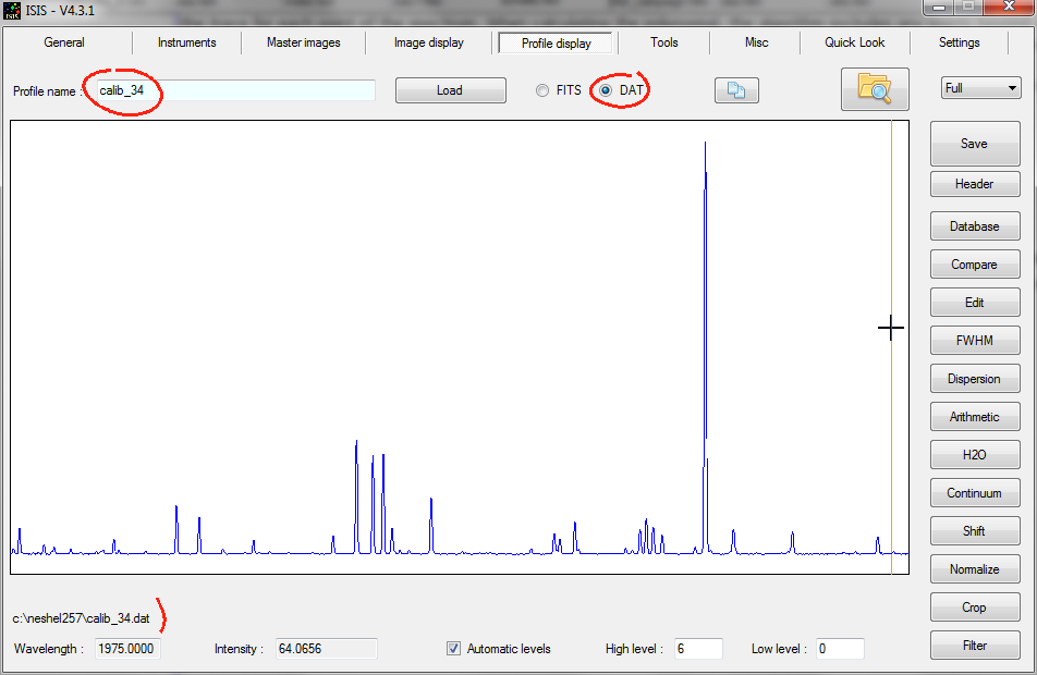
Signal distribution along spectral Thorium-Argon lamp order #34 (for example).
7.
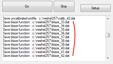
Computation of blaze function
Blaze
function, distinct for each extracted order, is a smoother
version of tungstein lamp raw spectrum. ISIS applied a gaussien
convolution for this. The blaze function represent the relative
spectral instrumental response for a given input spectral flux distribution
(here from an incandescent lamp). All science spectra are divided
by the blaze functions, saved on the disk as a ASCII files, named
"blaze_xx.dat":
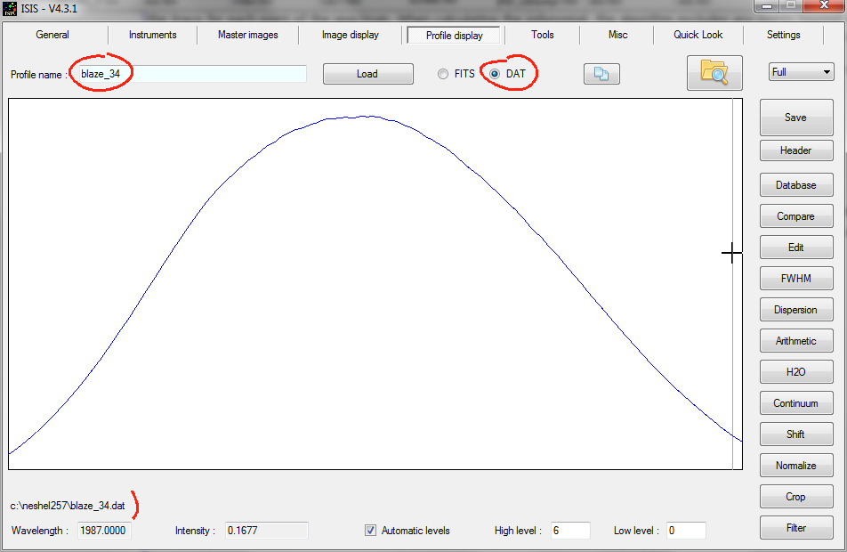
Example of blaze function for order #34.
The actual calib_xx.dat
(thorium-Argon) sequence is divided by the blaze function.
8. Evaluation of spectral dispersion solution
Now, ISIS use the "calib_xx.dat" spectra of Thorium-Argon lamp for compute the relation between pixel number along the dispersion direction and wavelength (the dispersion law (or dispersion solution), one for each order).
First, we etablish
the link between internal dispersion solution (pre-computed
by using fundamental grating equation, optic focal length, pixel
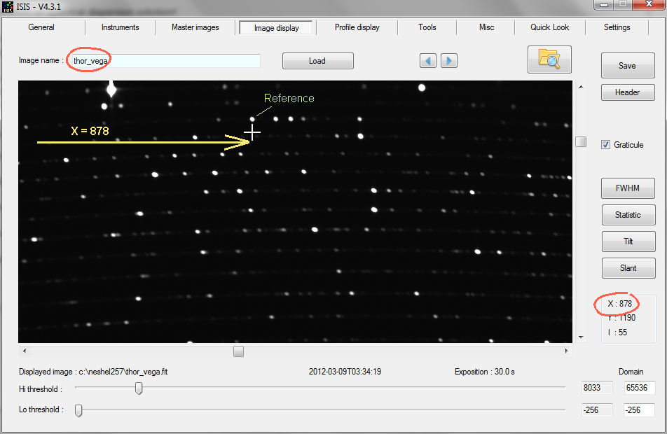
size, ...) and the observed X-coordinate of à Thorium-Argum at a
given reference wavelength. In the example below, the reference
wavelength is located in the order #34, at 6563.906 A and the measured
position is X = 878 (nearly):
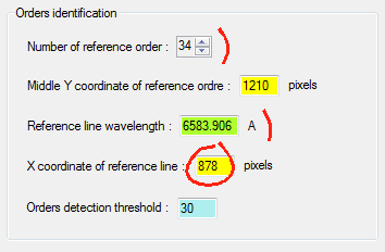
These parameters are given in the eShel Setup panel dialog box. Here the reference spectral line concerned for the example:
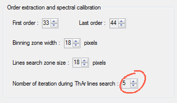
The dispersion equation of earch valid order "xx" is determined from "calib_xx.dat" spectral profile (ThAr spectrum). The used lines for this operation are identified on the file "line.lst" (stored in calibration subfolder).
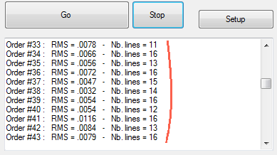
The position of the observed lines (in pixels) are measured by a gaussien fit method. Then, a polynomial dispersion is evaluated for each order (3th degree coefficient polynom). The RMS ajustement error is evaluated. The procedure is iterative. For a given line, if the actual computed wavelength varies by more than 1.4 x RMS from true wavelength, the line is rejected for the next iteration. Here, how to fix the number of iteration:
The OC_xx.dat ASCII files contain the difference between the catalog wavelength and the computed wavelenth by using dispersion solution:
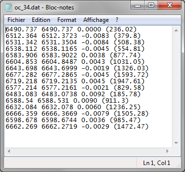
IRIS return also the RMS error of dispersion solution in angstrom:
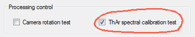
If you select the option "ThAr spectral calibration test", the program stop here. You can then see positions of the lines used by ISIS (image check2.fit):
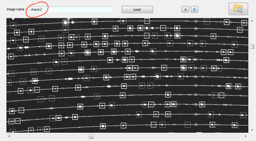
Dotted
rectangles corresponds to wavelength of starting list, the plain
rectrangles identify the actual used lines for calibration.
9. Extraction of profile from science image
To extract the raw science spectra profiles, ISIS uses the same procedure as for the calibration images: geometric correction, cropping of a sub-image per order, backgroung subtraction, optimal extraction of profiles from 2D sub-images. The raw spectral profiles (in pixels and digital count) are named # n_m.dat, with "n" the index of input image and "m" the order number:
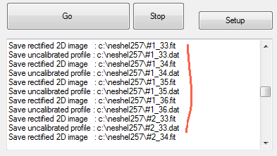
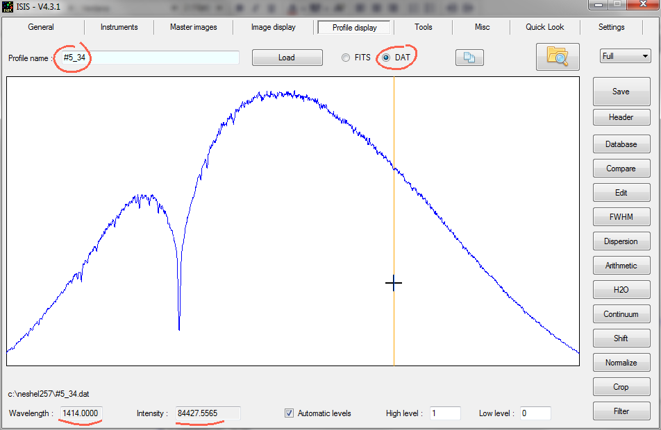
Raw
spectrum of order #34 extracted from input image #5. The wavelength
axis do not represent true wavelength, but pixel unit.
10. Addition
of individual spectral
The individual raw spectral profil are now added. Two methods are available.
If the option "Sigma-clipping" is selected:
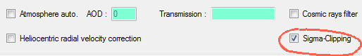
ISIS equalizes the intensity of all spectra of the sequence to add, then performs an addition with sigma-clipping rejection method: points of the spectra sequennce that deviate more than 5-sigma of the mean for a given spectral sample are rejected from the final sum. The procedure is iterative. The sigma-clipping method is more effective than the number of individual profiles is large (5 or upper).
To add less then 5 individual spectra or if the intensity between the spectra is very fluctant (or for a variable integration time along the sequence acquisition), you can choose weighting profiles addition. In this case, the option "Sigma Clipping" does not be selected..
The summed spectra (one for each order) are saved under working directory.The adopter generic names for these intermediate file is "calib_xx.dat" (xx = the order index).
Note: The calib_xx.dat contain is
divided by the blaze function of the corresponding order.
11. Spectral calibration and response correction
By using dispersion solutions, the "calib_xx.dat" are wavelength calibrated. ISIS convert the pixel interval into equal wavelength interval (linerization along the spectral axis) and redistribuate the flux along the wavelength by using spline interpollation. The commun base step value along wavelenth is 0.05 A.
If the instrumental response of each order is provided, the individual spectra calibrated in wavelength are divided by the corresponding instrumentale response.
Similarly, the spectra are divided by the atmopsheric transmission if this is requested (the atmospheric transmission is then calculated automatically from the AOD index - an access to internet is mandatory).
The intensities are then normalized to unity for the spectral range between 6620 and 6635 A (these values are hard coded in ISIS).
Finally the spectral range of each order segment is bounded by the values given in the ASCII file "del_lambda.lst", if it is present in the calibration files directory.
The result is saved under the name "calib_xx.dat" (the intermediate raw specra are lost for reduce the volume of intermediate files on the hardrive).
12. Fusion of segment order
The segment orders are combined for synthesis a full spectral wavelength range continuum spectrum.
The result is divided by a Planck function corresponding to a black body at 2750 K (typical color temperature of eShel calibration white lamp) if the instrumental response is global (not a response order by order).
The individual order are saved in files under the name "_objectname_yyyymmdd_fff_xx.fit", where xx is the order number.
The merged order version of the spectrum is saved under the name "_objetnamne_yyyymmdd_fff_full.fit".