ISIS
Version
5
Guide for
process LHIRES spectra
1. Purpose
This tutorial is a guide to learning ISIS especially for the processing of spectra taken with Lhires III spectrograph. However, this guide contains numerous practical information on the use of ISIS, in particular a description of the new features of version 5. Even if you do not operate the Lhires III spectrograph, reading and implementation of the proposed exercise can be very beneficial. Raw images to achieve the processing can be downloaded (see link below). The organization of the paper is a short step by step learning, based on concrete examples.
Procedure for change ISIS langage interface.
2. First contact
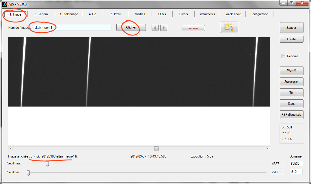
The guide is based on spectra acquired with the spectrograph Lhires III equipped with a 2400 lines/mm grating. We will process in particular a sequence of spectra of star Altair (Alpha Aql). Below, a raw image extracted from this sequence (compared to the original full format, the vertical size of the images has been reduced so that the download is not too heavy):
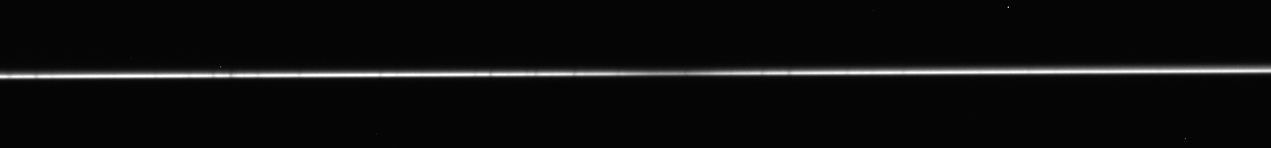
The star spectrum is the horizontal line that bar image. The image shows a portion of the spectrum centered on the hydrogen red line, Halpha, at wavelength 6563 Angstroms (6563 A).
The spectrum has been made with a spectrograph Lhires III 2400 lines/mm mounted at the focus of a old good F/10 Celestron 8 (D = 200 mm), with that antique orange color, but still fully functional:
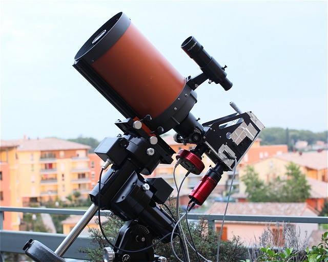
Acquisition software is AudeLa (also used for the guiding function, provided by a camera Atik314). The camera used for acquire spectra is a model Atik460EX, equipped with a relatively large format detector and displaying good performances, including a high quantum efficiency for this price (see here for more details). CCD pixels are very small, 4.54 microns. Unnecessarily small for our configuration in fact, so I decide to acquire the spectra in 2x2 binning format, bringing the effective size of the pixels to 9.08 microns (internal CCD 2x2 summation process during image reading). The spectrograph slit is 23 microns wide, which gives a resolving power of about 15,000 (i.e. the instrument is capable to resolve details of 6563 A / 15000 = 0.44 A). Finally, the exposure time is 90 seconds and I acquired in sequence 6 images of the spectrum of Altair, with the idea of ??adding their signal during ISIS processing
As mentioned in the introduction, I recommend to realize treatments described in this guide at the same time as you read the text. You will progress much faster and retain sustainable use all the tricks. It is almost mandatory to download all the raw data by clicking on this link:
The ZIP file is quite large: 7.3 MB Unzip the contents to a directory of your choice. However, I'll give you a tip for this exercise. The spectra were acquired in the night of 6 and 7 September 2012. So, a good idea (this is a personal approach) is to decompress the images in a directory named:
C: \ NUIT_20120906
Note that I am not a very supporter of paths like C: \ Documens and Settings \ ... \ ... \ ... There is no standard for storing and organizing data directories suggested by the designer of the operating system, far from being practical and rational in a scientific context. Make simple. There is no indication against access your working folder from the root C:, for efficiency. Optionally add a directory level, but not much from my point of view.
The construction of the directory name is quite logical. The word "night" (nuit in french langage) identify the nature of the data in your computer (again, you can choose a different name). It was then followed by the observation date (in US format U.S.: YYYYMMDD). Note that I adopted the separator symbol "_". Avoid absolutely the white character for folder and file names. This is technically a disaster (nothing looks more like two white and one follow white, for example), and you'll go crazy some users will want exploit scientific data. You have been warned!
The directory that you just created is called "working directory" in the ISIS jargon. Make a separate work directory by observation session. Here is the content for our tutorial:
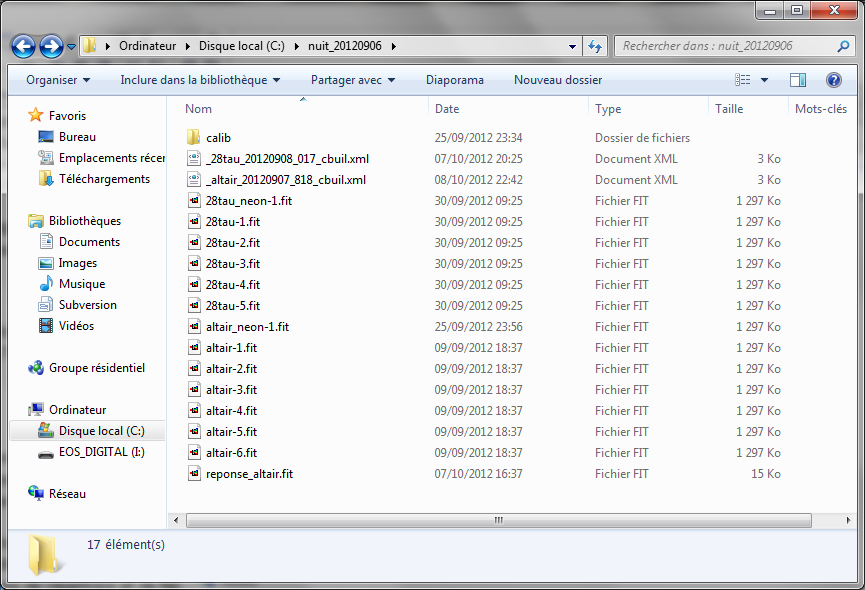
Note the presence of a subdirectory CALIB: it is optional. It contains useful data for calibrate the spectra and can be used without modification in a work session to another.
Now run the ISIS software.
Before processing your first spectrum, we have to make some adjustments. Assure you, for the most part, they are to do once. You will find your choice at the next work session with ISIS.
ISIS interface is composed of a series of tabs. Also note that you can enlarge the application window by dragging the lower right corner of the window with the mouse pointer.
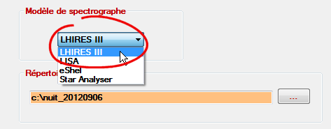
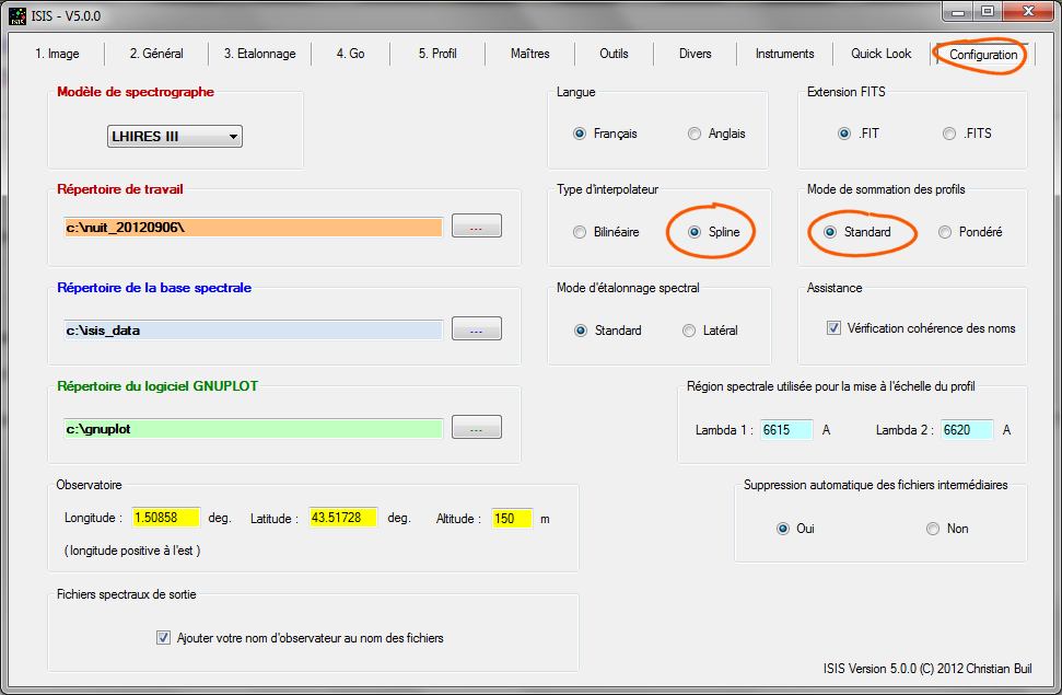
Open the "Settings" tab. In the section "Model spectrograph", select LHIRES III, since we are process data from this model.
Then, specify the path of working directory (or folder). Here i c: \ nuit_20120906 (you can enter letter in uppercase or lowercase, it does not matter).
Finally, provide numerical values ??for fields "Lambda 1" and "Lambda 2" in "Spectral domain used for profile scaling", respectively 6615 and 6620 values??. These are wavelengths are in angstroms. They define a range in your spectra where ISIS calculate intensity for normalise the spectra (scaling). You will see the effect later. We choose an area if possible without spectral lines. Use the values ??that I propose.
Here the actual look of "Settings" tab:
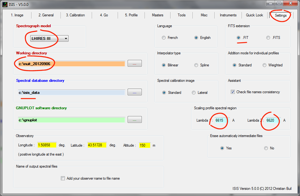
Note that the ISIS database is installed (c: \ isis_data). It is a folder that contains a variety of useful spectra for the time of spectra calibration, we have the opportunity to see. Installing the ISIS data base is a PRIOR important. If you have not already, check out this page which gives you the procedure.
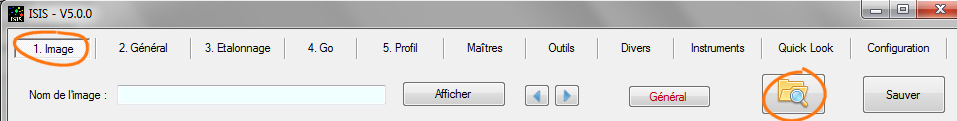
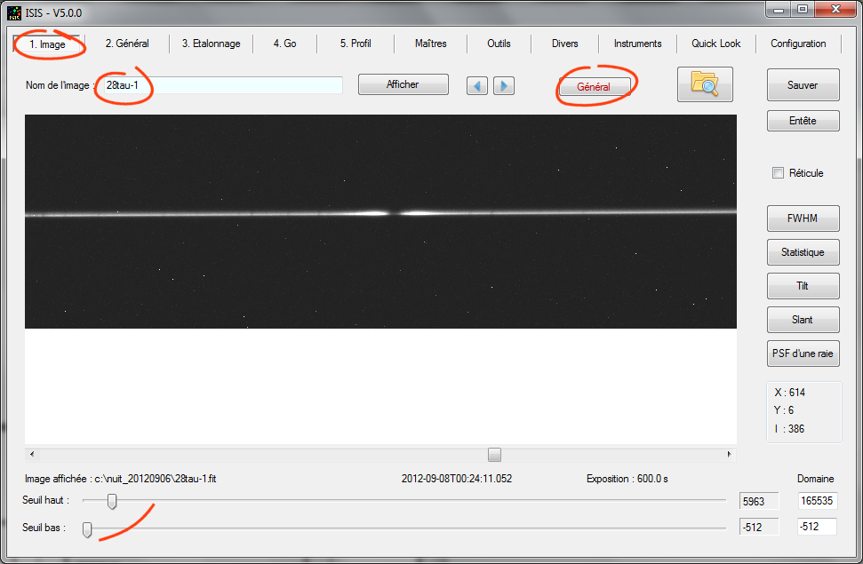
The file name in the sequence of images to process is altair-1.fit, altair-2.fit, ..., altair-6.fit. We will view the contents of these files. For this open the "Image" tab (on the left of the interface), and then click the folder and magnifying glass icon :
Select the file "Atair-1" and then click OK in the standard Window file select dialog box. The image "altair-1" is displayed automatically:
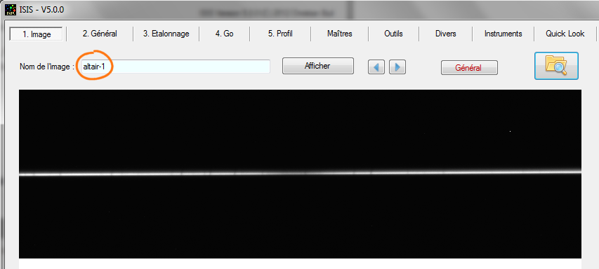
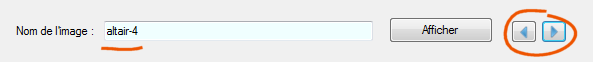
Note that the name of the image is automatically copied into the "Image Name" field at the top of the window, but not the file extension. For keyboard experts, you can enter here perfectly the name of a valid FITS file, then click on the "View" button to view the contents (or <Return> from the keyboard).
You can adjust the display contrast by turning the sliders at the bottom of the window.
Tip: If you double-click with the mouse in the circled areas shown in the figure below, the visualization thresholds automatically adjust to a typical value for the current spectrum:
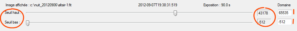
Take the opportunity to resolve the sliders excusion dymanic. The actual values shown are typical. It is possible to indicate negative threshold values, very useful to distinguish the image backgound of, often too dark without it.
Small "arrows" buttons can move forward in the sequence of images (recall, we have 6 Altair images). The image displayed automatically.
You must stop of the image name structure. It is critical point to efficiently exploit ISIS and quickly process your spectra.
In the file name in disk are::
altair-1.fit
altair-2.fit
...
...
altair-6.fit
When you specify a file name you never to add the extension. ISIS adds extension for you in the background.
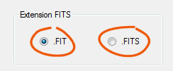
Note: Some acquisition software produce images with the extension ". FIT", others with the extension ". FITS". You can specify this feature in "Settings" tab:
If you forget the extension, the name itself is the example is: altair-1.
Starting from the right, the name is composed of 3 parts:
(1) an index which designates the row of the image in a sequence. ISIS still considers that the first index is "1". Image sequences are indexed in the follows maners: 1, 2, 3, ..., 12, 13, ...
(2) a suffix, which will serve as a separator between the "root" name and index. In our example the suffix is the symbol "-". You are completely free to choose the suffix, which can be perfectly composed of several letters. However, the single dash is a good idea if your acquisition software agrees: it's short, simple, easily identifiable.
Important Note: You can ignore the suffix after all ... In this case the images sequence is atair1, altair2, altair3 ... It is not at all recommended to do so. Suppose you have a sequence of star HD4523. If you do not suffix, your filenames in the sequence will be: HD4521, HD4522, HD4523, ... The result is unreadable and it is ambiguous. The star HD4521 exist, aloso HD4522, but which it is another star .... Such management of file names is very bad. All is clear if your individual filenames in the sequence are: HD452-1, HD452-2, HD452-3, ...
(3) a root name here "altair". We must choose carefully. Avoid long names, it is useless. Except for the brightest stars (Vega, Altair, Deneb, Sirius ...) avoid a root name as "Cor Corali." Typo risks is considerable, it is difficult to enter from the keyboard, it is not always recognized by professional databases, this is not scientific ... Prefer HD numbers or ultimately, the Flamsteed designation (zeta_oph, DeltaCep, ...).
Even if it is managed by ISIS, also avoid white character in names (to be replaced by the character 'undescore', "_").
ISIS often requires as a parameter the name of a generic sequence. The generic name is composed of the fusion of the root name and the suffix. In our example, the generic name is "altair-".
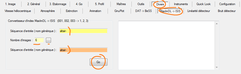
Note for users of the MaximDL software. This software cal image sequences as follows: altair-001, altair-002, ..., 013, altair, altair-014,... while ISIS expects the sequence altair-1, altair-2, ..., 13-altair, altair-14, ... (more logical and universal!). You can convert MaximDL names into ISIS system automatically via the "Misc" tab, then the sub-tab "MaximDL -> ISIS" :
In the data provided for this tutorial, you'll find very specific files. Their name finish with .xml extension. The computer experts will recognized the signature XML format file. We can arrange hierarchically data in these files for example. This is one of their major interests.
Whenever you use ISIS to process a sequence of spectra (or individual spectrum), it keeps trace of this processing, saved in a XML file. Everything that is needed to replay the processing days or years after the first processing is contained in the XML file. This possibility is of course very interesting for analysis and make adjustments for example. I have already processed the Altair sequence and I have added the corresponding the configuration file in the distribution file for this guide. For now, I suggest you replay the complet processing by using the XML file. This will already very informative!
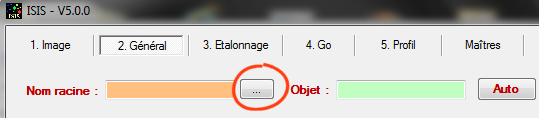
Go to the "General" tab. This is the control tower at ISIS. Click the "..." button following the "Root name" field:
Choose XML type file in the selection window that opens. A file of this type is associated with the Altair spectrum:
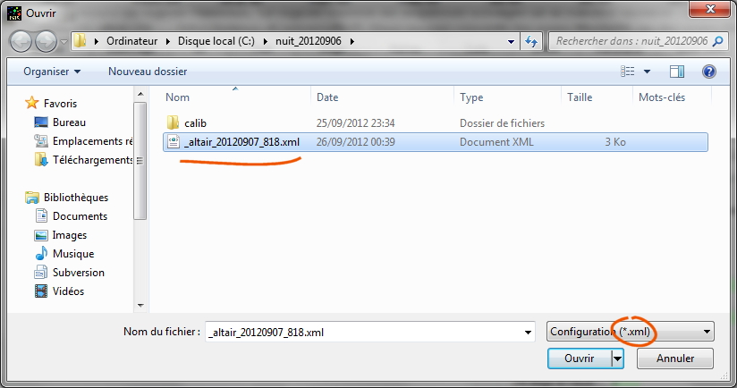
Open the file.
Tip: The contents of the XML file in question can be consulted with the help of your internet browser:
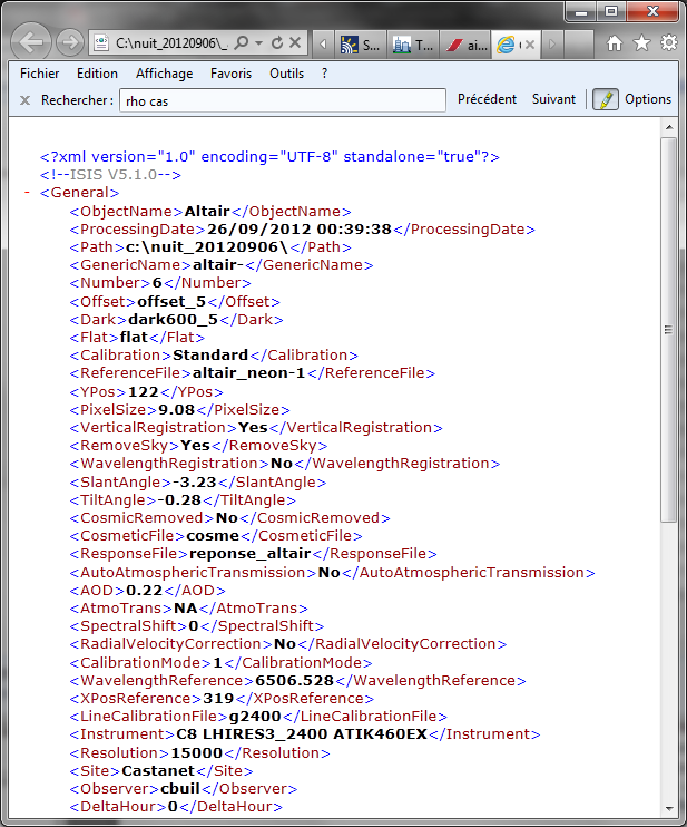
After opening the XML file, numerous ISIS fields interface are automatically completed (or pre-filled). Note that some fields are virgins of information (this is the way in ISIS to indicate that optional field is not used):
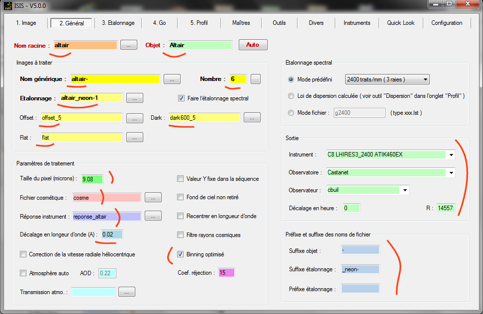
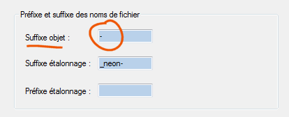
Note that the general suffix used in ISIS is specified in the XML file we just opened, here a simple dash "-" (field "Object suffix" down the window):
Everything is ready for an immediate process Atair sequence and extract the spectrum. Open "Go" tab and click directly on the "Go" button:
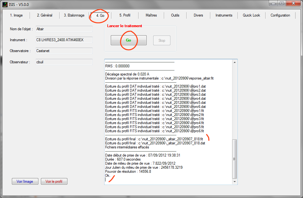
The calculation takes only a few moments. The result is the spectral profile "_altair_20120907_818.fit" stored by ISIS in the working directory. The structure filename result is immutable. The name always starts with the character "_". Then, the object name (this is not necessarily the root name). Finally comes the start date of the observation in the format AAAAMMDD_FFF with FFF, the fraction of a day.
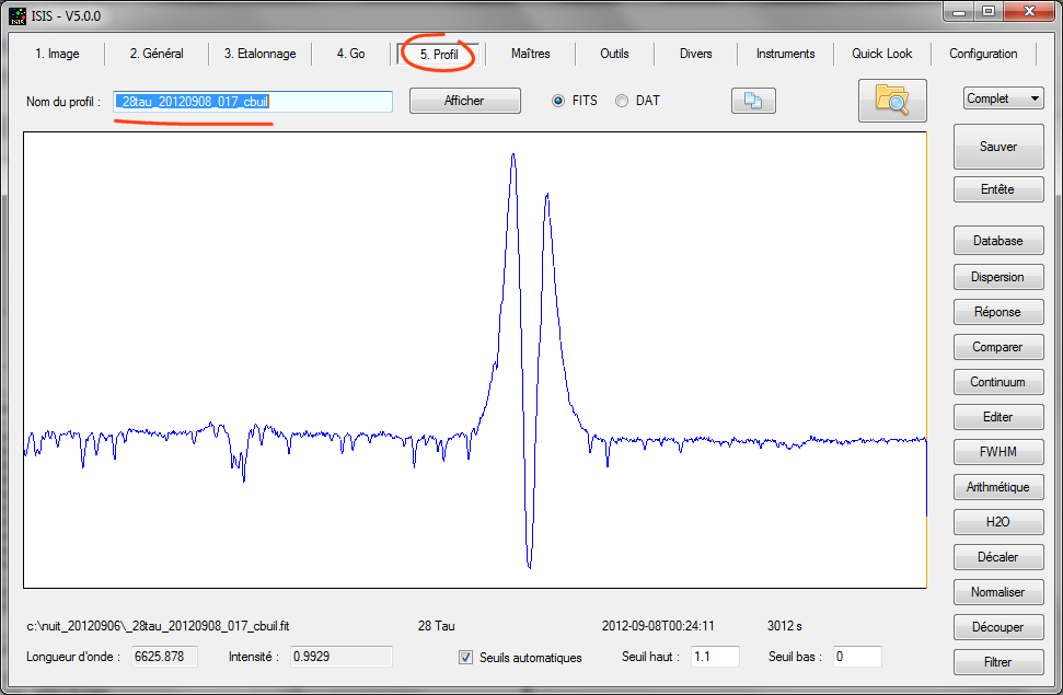
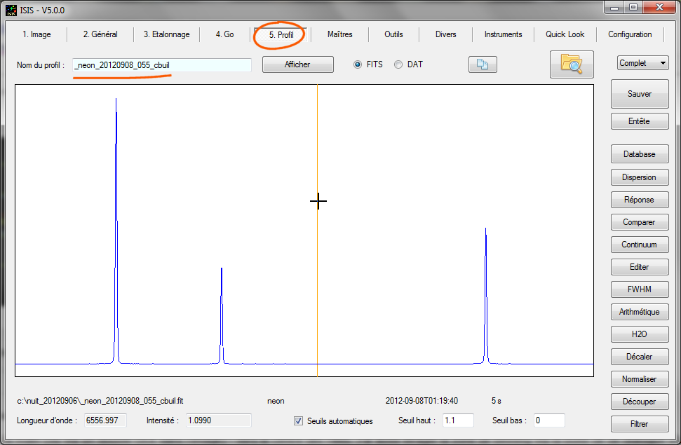
To view the profile, you can open the "Profile" tab, then click on the "Display" button. But there is quicker: just press the button "Display profile" at the bottom of the "Go " tab:
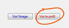
This opens the "Profile" tab and displays the calculated spectrum directly:
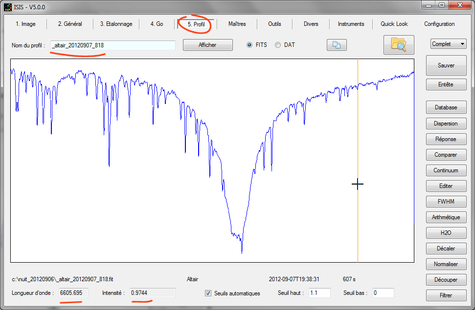
The spectrum is calibrated in wavelength. When you move the cursor horizontally, the actual wavelength value that appears at the bottom of the tab change. The spectrum is also corrected for instrumental response (the instrumental response contain flux distortions in stellar flux induced by variations of atmposhéric transmission or spectral sensitivities of the instrument. The spectrum is also normalized to unity around wavelengths Lambda Lambda 1 and 2 (adjusted in "Settings" tab).
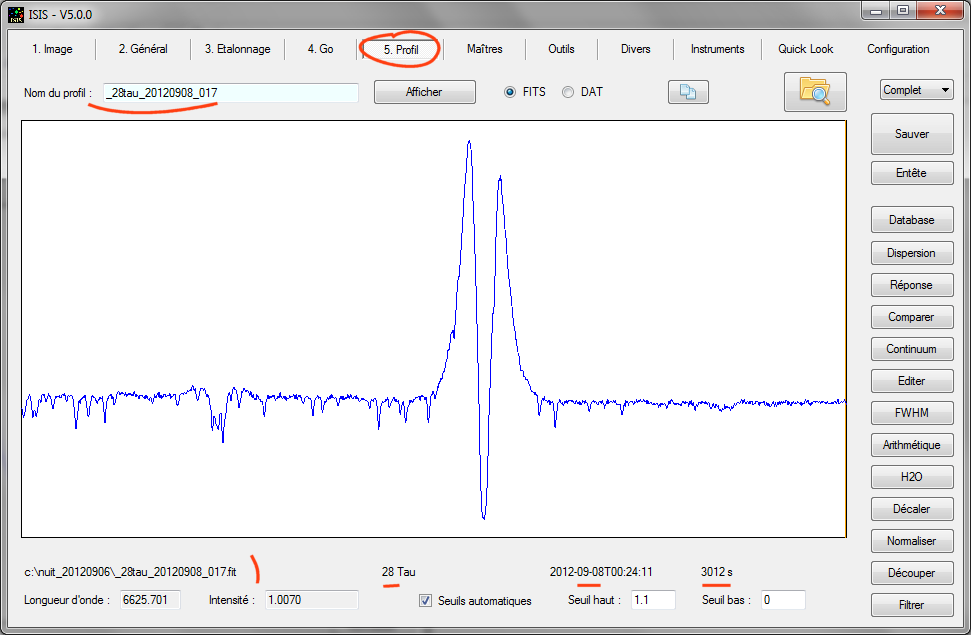
It is instructive to process the spectrum of another star performed during the same session. I chose the example of the spectrum of 28 Tauri, a Be-type star (star B shows the hydrogen lines in emission). We have obtened five spectra images, each exposed 600 seconds. The XML file processing is available for this star in the working directory (_28tau_20120908_017.xml). Load in the usual way, as described above, from the "General" tab.
Tip: You can open a dialog box for selecting an XML configuration file in ISIS by clicking on either one of the two the following buttons:
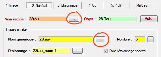
Here the state of the "General" tab now. It shows the differences in relation to the Altair sequence processing:
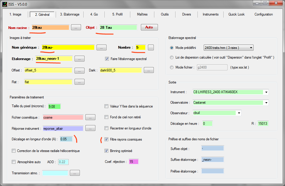
For the most part, the differences with the Altair processing correspond to bold enhanced fields. Logically, the differences between Altair and 28 Tau settings concern the name of the raw file, the "catalog" name of the object and the number of acquired images. It there is very little information to provide ISIS to move from one star to another when processing a full session. It is a guarantee of ease of use and reliability (limitation of error risk).
Open the"Go" tab and start the processing ("Go" button). Here the result:
3. Spectra calibration
Before performing the routine processing with ISIS, three preliminary operations are carried out:
(1) Calculate the master images offset signal (or bias), the thermal signal and flat-fied.
(2) Select a method for producing the spectral calibration, i.e. attaching a wavelength at each measuring point as accurately as possible.
(3) Extract the global instrumental response, i.e. the way in which your instrument attenuates the objsect signal in function of wavelength. The ideal instrument would be that offering a flat response, mitigating the same way all wavelengths acquired. There not count! The reasons for a non-uniform response in wavelength are too many: the optical transmission of the telescope, the spectrograph, the spectral response of the detector (the quantum efficiency) and also atmopsheric transmission, which is regarded as part of the instrulental response in ISIS in most situations.
So, first we need to build master images. These are reference images eliminate bias and distortions induced essentially by detector and its environment. The procedure is quite similar to that used in deep-sky imaging. Note that masters images are optional. . If you can't have for one reason or another one of these reference images (or master) you can leave the corresponding fields blank in the "General" tab. Avoid using this trick: these reference images are really needed to produce high quality results. Go here for detailed explanations on how to obtain master images from ISIS.
Since we start from scratch here, so that the demonstration is complete, looks "General" tab now:
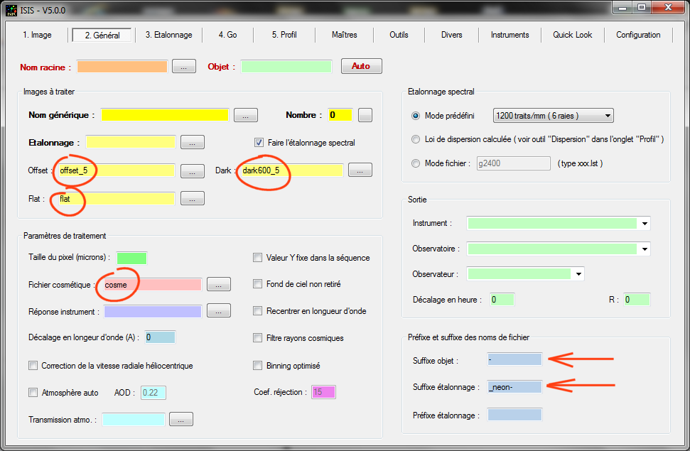
Fields corresponding to the master images have been completed. We took the opportunity to define some suffixes (separators with index in a sequence).
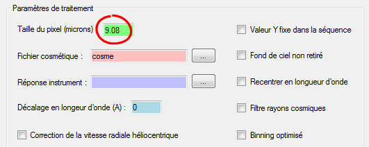
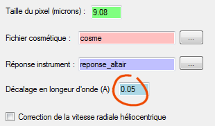
It is important to define a geometrical parameter of your instrument: the detector pixel size in microns. For Atik460EX, the native pixel size is 4.54 microns. However, the camera is operated in 2x2 binning. In this case, the pixel size is 2 x 4.54 = 9.08 microns, so
Indicatet o ISIS the type of instrument and who you are. This information will be automatically entered in the FITS header files results. This is fundamental for the scientific exploitation. Here's done:
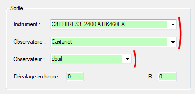
Try to be both comprehensive but compact. For the instrument, indicate in the order the type of telescope (Celestron 8), the type of spectrograph (LHIRES III equipped with a 2400 lines/mm grating ) and the type of camera (model Atik460EX). Also specifies the name of the observatory as well as your name observer (cbuil for Christian Buil, for example).
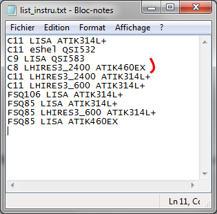
Tip: You can create a collection of instruments, observatories and observers. For example for the instrument, create a text file named "list_instru.txt" (the name is imposed) in the ISIS installation directory (save the file in the same folder as "isis.exe") in the style:
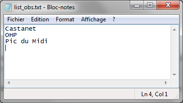
or fot the observatory - a file named (mandatory) "list_obs.txt"
and a list of observers, the file "list_observer.txt."
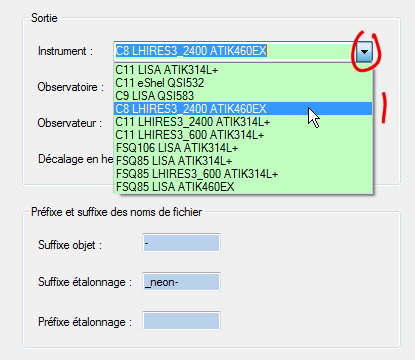
You can now easily select the configuration from the "General" tab:
ISIS offers a number of assistants to help you during processing. The content of assistants may be different depending on spectrograph model: LHIRES 3, LISA ... Indicate your intrument now to ISIS from the "Settings" tab:
Tip: If your spectrograph is not in the list, select the template LHIRES III, an option that provides the most general utilities in ISIS.
We now make spectral calibration of Altair spectrum (from the sequence altair-1, altair-2, ...).
Display the content of first image of the sequence (for example) from "Image" tab:
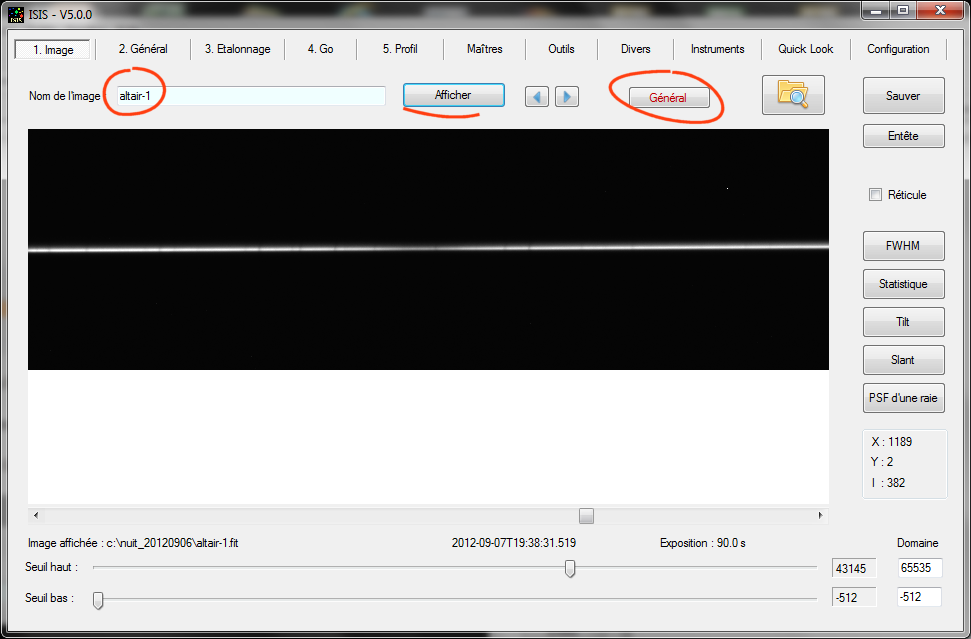
If you click on "General" button in the upper part of the "Image" tab, ISIS switches directly to the "General" tab and automatically filled some field for you:
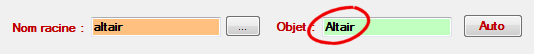
ISIS can not however define itself the content of the "Object" field. This is the name found in catalogs for identify the object. It should be here at the same time simple and precise in choosing the name. The same object can have multiple names, be listed in several catalogs. Use the names of stars if they are brilliant and well known. Prefer the identification of major current catalogs (HD5987, NGC2900, WR144, ...). Note that this is the only place where ISIS is sensitive to case (uppercase or lowercase). In our example, we adopt the name "Altair", because it is a simple and well-known designation for Alpha Aql (if you ask the CDS, the name Altair is recognized, it is a good test):
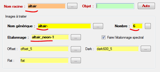
ISIS understood that the root name of your image file input is "altair". The number of images in the sequence has been automatically calculated. ISIS has also
well found in the working directory of an image for specral calibration "altair_neon-1".This latter contains the spectrum of neon lamp inside the spectrograph Lhires III, made just after shooting of six images of the sequence "Atair-xxx". you can look the image conteain from "Image" tab if you like:
ISIS automatically constructs the name of the calibration image by adding the root name "Altair" and calibration suffix "-_neon", but also an index number that is always "1" in this case. This is an arbitrary choice. It is assumed here that you are likely to have acquired a sequence associated with the neon lamp during Altair observation (altair_neon-1-2 altair_neon altair_neon-3, ...), but only the first frame of the sequence is considered here. You can well change the contain of "Calibration" field if you find it necessary (and write for example altair_neon-2, my_calibration_ image, ...).
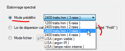
In the observed spectral range, the detector recorded only three spectral lines of neon around the stellar Halpha line. These lines are located at wavelength 6506.53, 6532.88 and 6598.95 A. ISIS offers several modes for spectral calibration. For the présent situation ( Lhires III configuration, 2400 l mm grating and three neon lines available), ISIS of a wizard that makes it simple calibration. We will see another method, more universal, suitable for all spectrograph at the end. For now, in the "General" tab and "Spectral Calibration" section, choose:
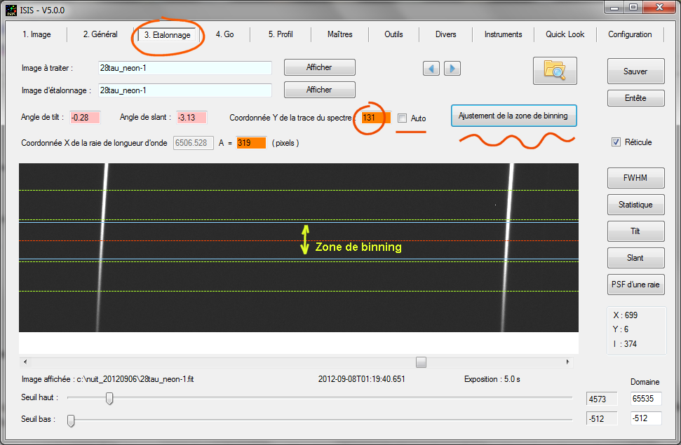
At this stage, the "General" tab dipose of enough information for process the spectrum. Open "Calibration" tab (just to the right of the "General" tab).
Altair-1 image is automatically displayed when the tab "Calibration" opens, you do not have to intervene more than that (possibly act on the sliders contrast):
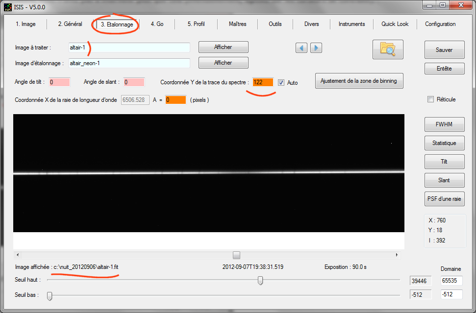
More specifically, ISIS displays the first frame of the sequence to be processed. Note that the names "altair-1" and "altair_neon-1" were copied for you from tab "General".
For further processing, ISIS needs the approximate vertical coordinate (in pixels around 5 or 6) of the spectrum trace of the spectrum. This measure must be taken to middle of the spectrum image (relative to the horizontal axis). It is possible to find this amount from the Y coordinate of the mouse pointer by moving it to center of the spectrum and reporting the value found in the "Spectrum vertical coordinate" field. You can go faster by double-clicking on the image with the cursor positioned on the middle of the trace. There are even simpler: if the "Auto" checkbox is enabled, ISIS calculates for you the next time "Calibration" tab is open. Here we have Y = 122 (the origin of coordinates in the image is taken at the bottom left).
Now, measure the inclination of the spectrum relative to the horizontal axis of the image (angle of tilt). With the mouse, define a rectangle that encloses the spectrum (drag with the left mouse button), then click on "Tilt" button:
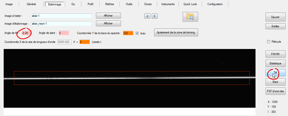
ISIS find a tilt angle of -0.28 ° (deviation from horizontal).
Superimpose on the the image of a grid that specifying binning areas used to construct the spectral profile and defining the sky calculation areas.
Check "Graticuke", then press the "Binning zone adjusting" :
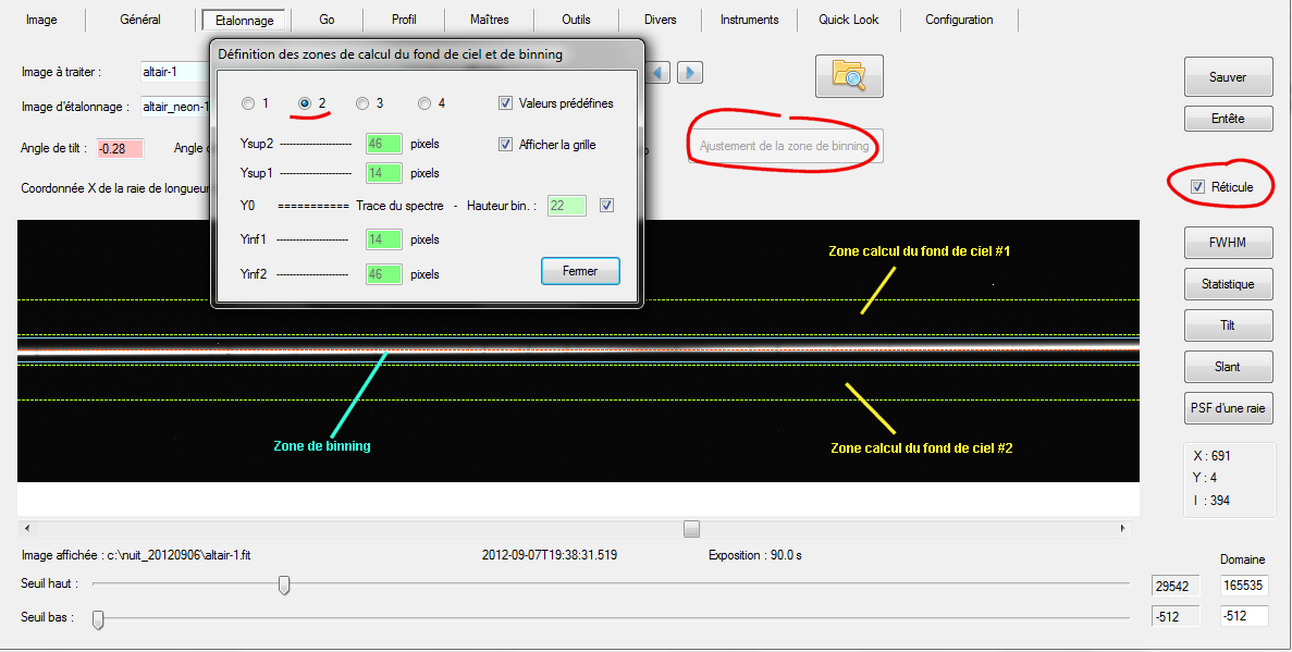
Note: the binning area (part where the pixels are summed along a vertical axis to construct the spectral profile) is flanked by two blue lines (22 pixels high). You can change the values interactively and see the effect in the image. For convenience, I chose number 2 preset values, suitable for case treated.
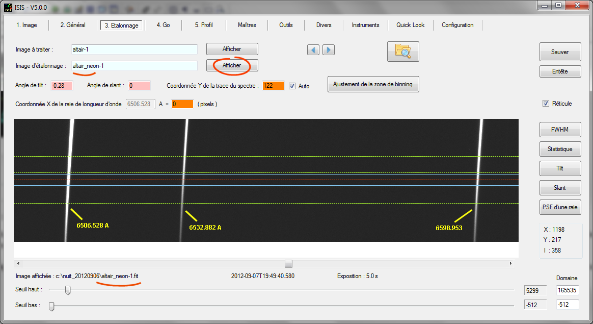
Now display the neon calibration spectrum (click on it to "Display" button in regard of "Calibration image" field). Expand the window application to see three the neon lines available for spectral calibration (and continue to keep the graticule displayed):
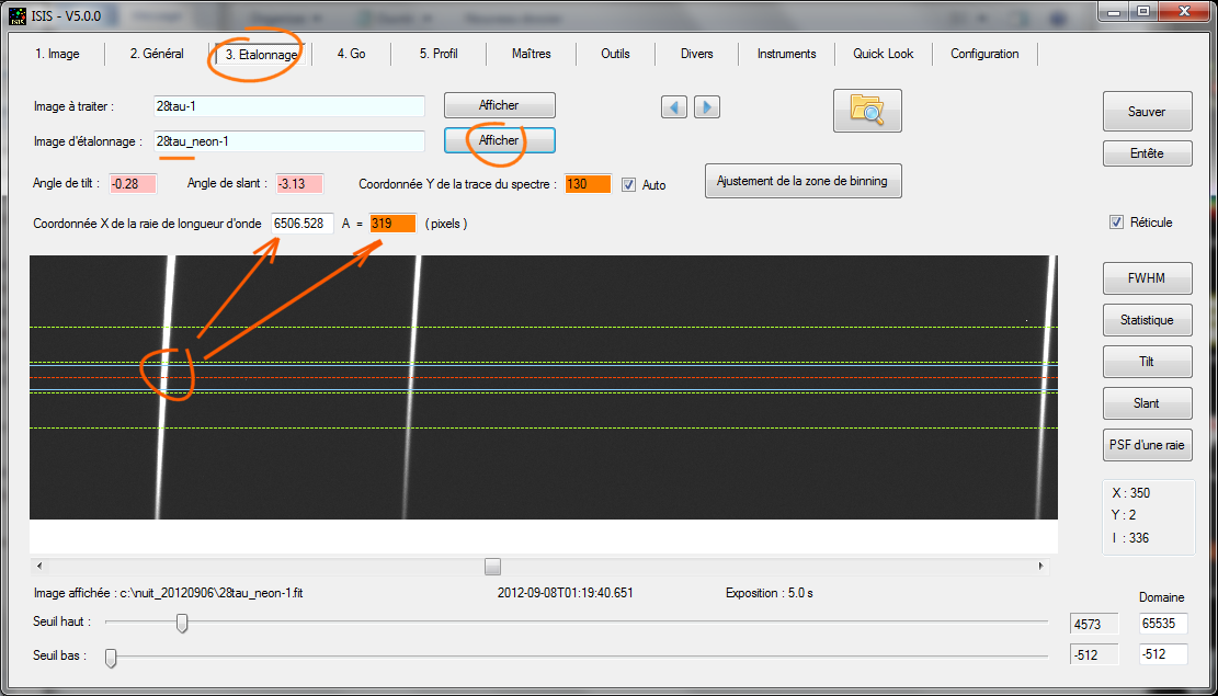
With the mouse pointer, double-click where the neon line at wavelength 6506.528 A intercepts the red reticle. Horizontal coordinate is reported in the field "X coordinate...":
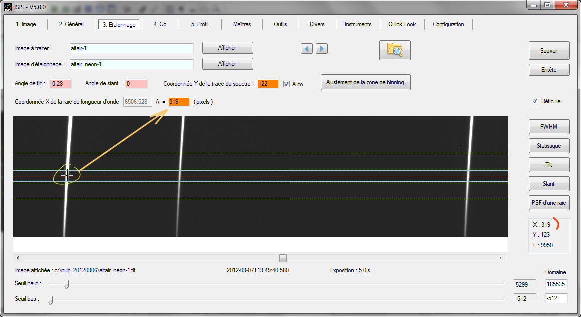
The coordinate of the line at 6506.528 A measured along the spectral axis (X axis) is equal to X = 319. ISIS need only an approximate value (+/- 3 or 4 pixels precision). The software will refine itself during processing. Note in passing that the meaning of the double-click with the mouse changes depending on the type image displayed (spectrum image to process or neon image).
The final information to provide isthe angle of inclination of neon lines with respect to the vertical axis (called slant angle). Define a selection rectangle of moderate height around the central line (for example), then click the "Slant" button:
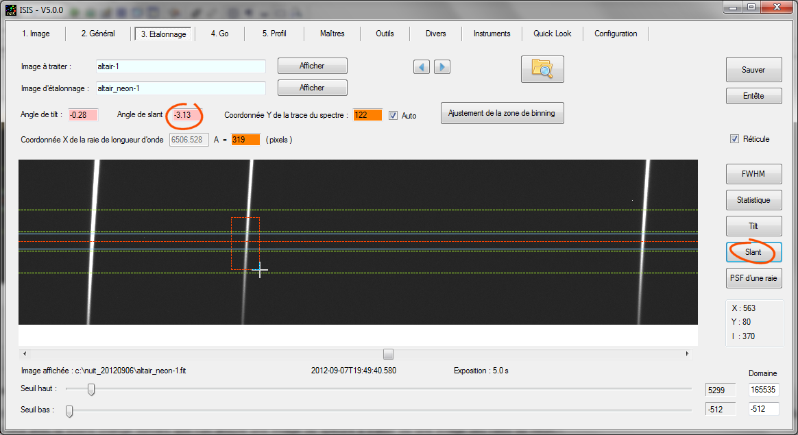
ISIS uses the upper and lower limits of the rectangle to calculate the value of slant angle of slant. The width of the rectangle does not influence the result, but it must howeve be wide enough to cover the line in its upper and lower parts. Depending on the shape of the rectangle, the result may vary: do worry, a difference of a few tenths of a degree will not change here basically the result of your processing. We find approximately -3.1°.
Important Note: During a work session, it is unlikely that all numerical values that we are now entering change radically. "Calibration" operation may be practically skipped when processing spectra following. A small control of the Y coordinate for the trace of the spectrum, however, does not wrong. If you check the "Auto" option, the calculation is done in the background when opening the "Calibration" tab. You have nothing else to do so as simple visual inspection.
You can now process your sequence of spectra. Open "Go" tab, then press the "Go" button. The calculation only takes a few seconds:
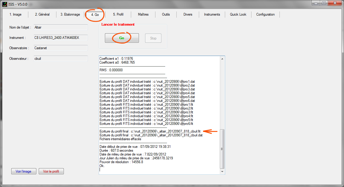
Note the name of the main output file, which contains your processed spectral profile, here:
_altair_20120907_818_cbuil
As noted above, the start character "_" is always added by ISIS. It allows you to distinguish the processed files in the working directory. Follow the object name (here "altair"). Next the starting date for the first image of the sequence in the format AAAAMMDD_FFF (FFF is the fraction of a day). ISIS add your name to observer (example, "cbuil"). It is not mandatory. This happens here because we have a special option in the "Settings" tab:
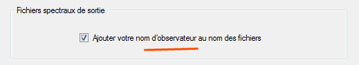
It is strongly recommended to select this option if you share with a community (database, observation campaign, ...). At the first look, the origin of the file can be identified. Think about making life easier for those who will exploit your spectra!
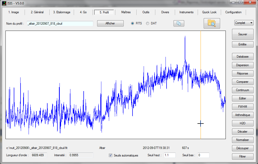
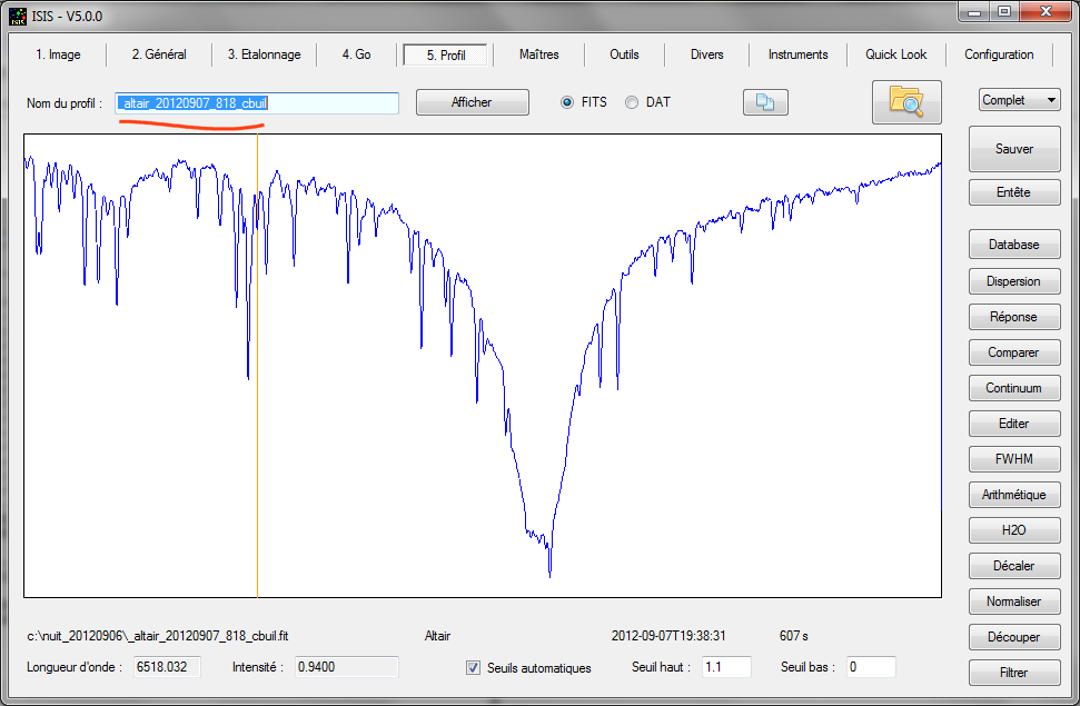
A simple way for display the result is a click on button "Display profile" of "Go" tab: clicking on the button "View Profile" tab from the "Go":
In this way the "Profile" tab opens automatically and the spectral profile calculated from all your original images also appear automatically:
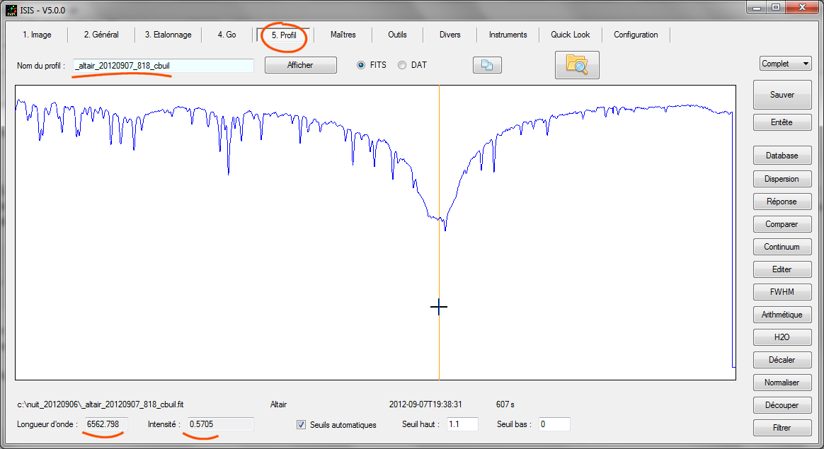
Note that the spectrum is calibrated in wavelength. The Halpha line center is well approximates at wavelength of 6563 A.
The choice of the processed type star at first is not trivial. Altair is clean of fine spectral lines. This type of hot star (spectral type A or B) are ideal for calculate the instrumental response. This is what we do now. Here is a rigorous method that I recommend ... This is the hardest part of the processing, which requires more handling. But there is nothing insurmountable as you go see, I think! In addition, remember that these operations are to do that from time to time only (not necessarily for each work session).
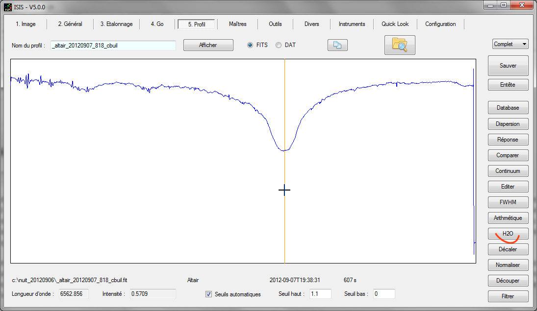
First, our Altair spectrum does not seem so bare that. It is encased in fine lines. These are actually rays of the atmospheric lines produced by water vapor (H2O). This telluric lines are called to distinguish them from stellar rays. To properly assess the instrumental response, it is desirable to erase these spurious. For this, the calculated Altair spectrum will be divided by a theoretical spectrum of water vapor. Unfortunately ISIS does not implement a automatic function for this operation. We'll have to do it manually, but it is not very difficult ...
Click "H2O" button present in the bar right in the "Profile" tab. A new window opens:
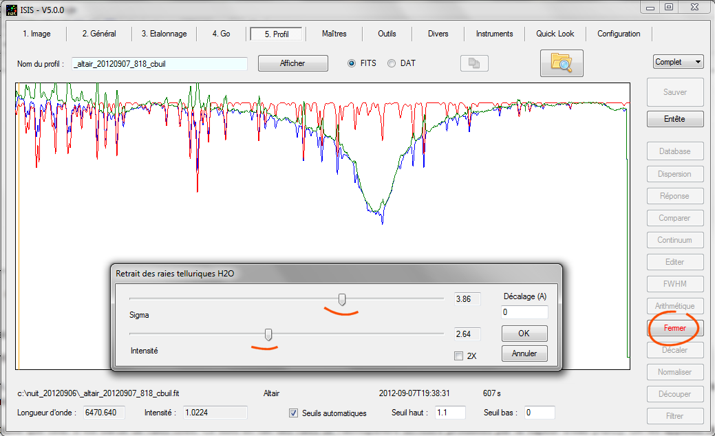
ISIS now shows simultaneously three profiles:
- Blue: Spectrum of your departure.
-
Red: The theoretical spectrum of the water vapor. You can change
its appearance by acting on the sliders in the dialog box (the cursor
"Sigma" rule th linewidth, the cursor "Intensity"
sets the depth). Do not hesitate to manipulate to see how the program
reacts.
- Green: The result of dividing the spectrum of the star
and synthetic water vapor spectrum present. This spectrum is
calculated each time you release the sliders for adjusting H2O spectral
lines shape.
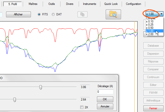
Often, to see the effect, enlarge a portion of the profile. This ability to detail a region of the spectrum is an important function of ISIS, available any time. Do here, for example:
Our goal is to erase the best telluric lines so as to keep the stellar continuum and the stellar lines only. It should here a little experience, but it comes soon as the result is very visual. For a nearly optimal result in our example::
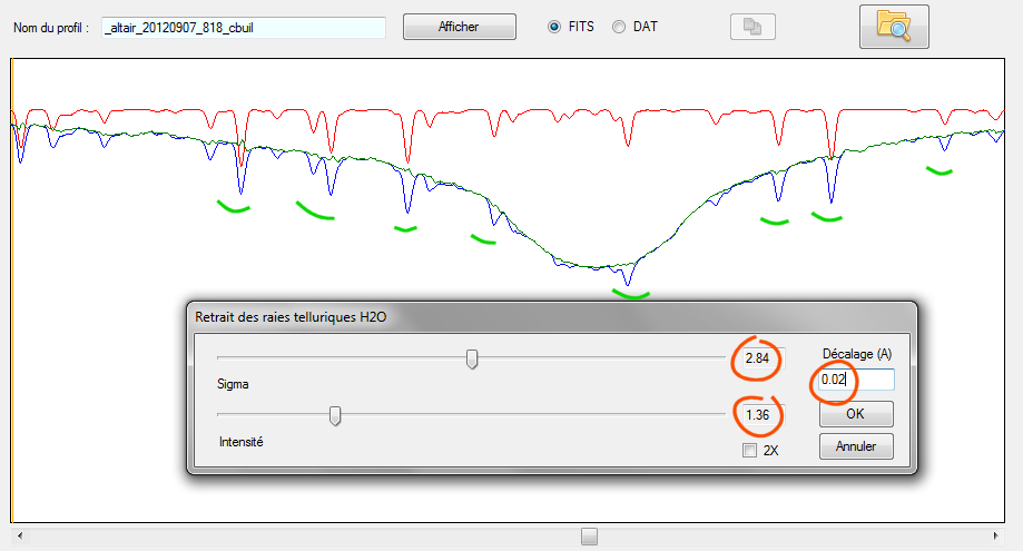
Note the absence of telluric lines in the spectrum plotted in green. This is the goal. To get the result just shown, it was also necessary to produce a slight spectral difference between the star and H2O spectra. Here, the H2O spectrum is shifted 0.02 A for superimposed on the best telluric lines on the star. Change this shift value (which can be negative) and see how the ration spectrum (in green) change. To confirm your entry, please <Return> ont the keyboard, or move the slider cursor slightly. The spectral shift can be caused by mechanical flexure between the time of you acquire the star spectra and instant of internal neon lamp acquisition.
For the present situation the spectral displacement of the observed spectrum of the star relative to the reference spectrum is very low here (it corresponds to a radial velocity of 1 km / s), but still detectable with the proposed procedure. Comparison of a spectrum containing telluric with HO synthetic spectrum is a powerful method This is why it is very important to know how to use the tool "H2O".
The value of "Sigma" is often a constant for your instrument. Unless a catastrophe on the side of the focus of the spectrum, the instrumental width your lines is always approximately the same. Ultimately, only the intensity is adjusted and optionally, a spectral shift.
At this point if you click the OK button in the dialog "Remove H2O tellurics lines", ISIS displays current spectrum as the result of the division of starting spectrum and spectrum H2O adjusted:
Telluric lines have been erased with good efficiency (residues on the left hand margin indicate calibration of lower quality in those parts of spectrum due to optical distortion: the spectrograph Lhires III is not calculated to cover as wide spectral area with this grating).
Tip: If you have a regret, if you want to start over, it is very easy to reload into memory and display the original spectrum. just click on the "Display" button at the top of the "Profile" tab:
![]()
We can see on the right side of the spectrum intensity falls to zero. This is a side effect of calculation. It is desirable to keep the significant spectrum part, both left and right. In other words it must crop. Click on "Crop" button. By positioning the orange vertical cursor make a double click on the edge of the left side of the spectrum you want to keep. The vertical cursor becomes black and thick. Then double click on the right limit (the order right or left can be perfectly inverted):
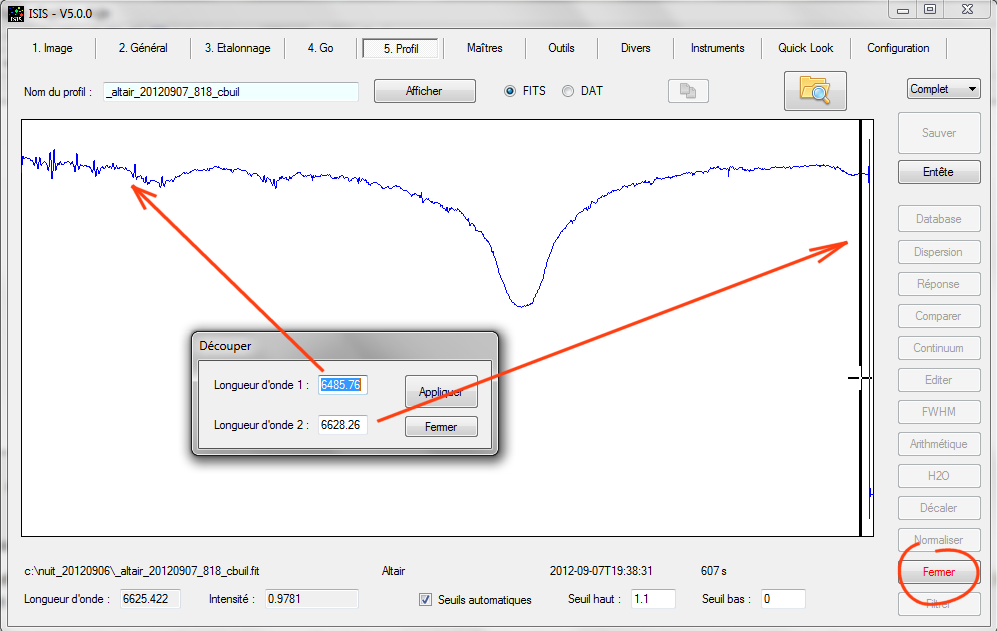
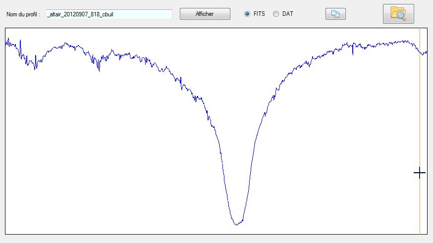
The profile is automatically cropped. Close window "Crop". Here is the result:
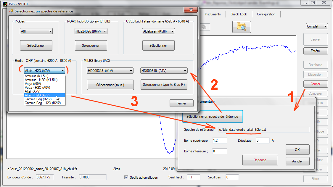
The instrumental response is obtained by dividing the observed spectrum by the real spectrum of the same object, or in any case, a spectrum of the same spectral type. ISIS database contains a portion of the Altair spectrum made with the Elodie spectrograph at the Observatoire de Haute Provence (OHP). Press "Response" button. In the dialog box "Instrumental response" that opens, click on "Select a reference spectrum" buttton. The database selection dialog appears. In the section "Elodie", select spectrum "Altair - H2O (A7V)" (a spectrum where telluric lines present in Elodie the data are removed). Finally, click the "Select" button:
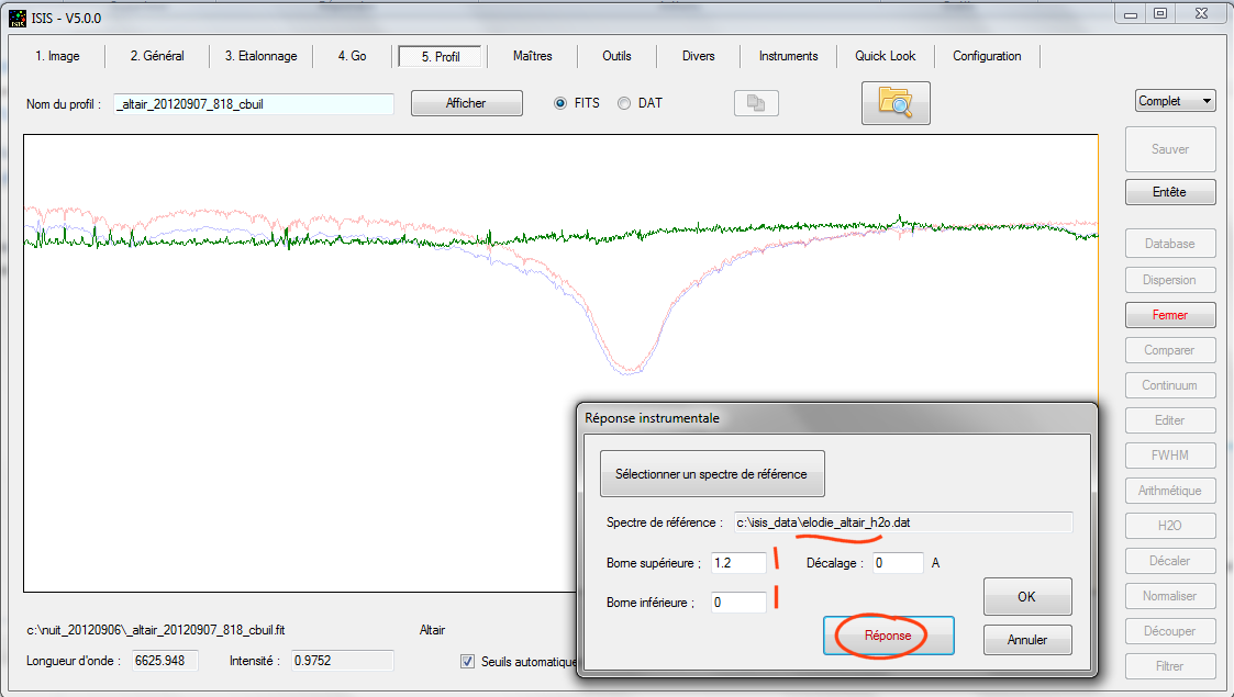
Click "Response" button" of dialog box "Instrumental response". Therefore, ISIS displayed on the same graph:
- Blue, the observed spectrum;
-
Red, the reference spectrum (that would normally return the instrument);
-
Green ratio: observed spectrum / reference spectrum, that is to
say, the instrumental response.
Look carefully at the red and blue profiles: there is a slight redshift between the two Halpha line. The reason is simple: these two spectra were
acquired at different dates, corresponding to a different radial velocity related to annual rotation of the Earth around the Sun. Must cheat a little here and shift
(translate) the Elodie spectrum is superimposed on the observed Altair spectrum. Here is the result:
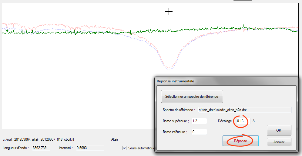
Proceed by successive trials validating, each time by pressing the button "Rsponse". By a simple visual examination found a shift of approximately 0.16 A. The accuracy here is sufficient. Click "OK" in the dialog box to keep the instrumental response (green curve, which becomes now the current profile in memory):
Rest assured, the result seems very noisy, but it is actual autoscale display that accentuates this appearance. In fact, all points of the ratio are close to unity intensity (move the cursor to realize). However, this noise is real and most importantly, it does not reflect the appearance of the instrumental response. The latter is a much smoother curve, which changes only slowly as a function of the wavelength. For compute this effective response, smooth the current curve. The most simple and effective way to do this is to use the tool "Continuum". Click
"Continuum" button located on the vertical list button at the right of "Profile" tab. In the dialog box "Continuum adjustment" that opens, simply to click on "Automatic # 2" button:
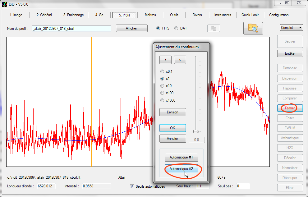
Red, you start profile and blue the corresponding smoothed profile. Close the dialog box by pressing the "OK" button. It remains only to saved in the working directory the instrumental response calculated as distinct spectral profile. To save the current profile to a file, press the "Save" button:
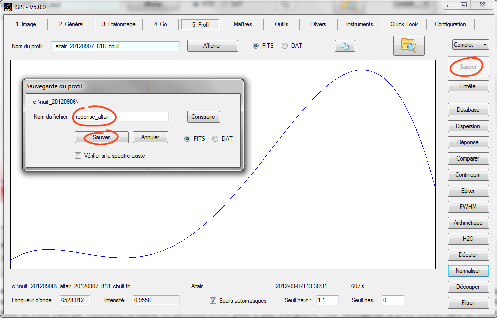
The given name is arbitrary. You have all the choices. Here, I chose to name "reponse_altair" because it is an instrumental response and I add the name of the star from which it was calculated (note that I never put the white characters in the names file!). Click the "Save" button. It is finished, the hardest part by far, you have your instrumental response (relative to an Elodie Altair spectrum, which we hope it reflects the true spectrum of this star, as if it were observed outside the Earth's atmosphere - this is already a good basis for work).
The instrumental spectral response will help us to refine processing of all spectra of actual session and probably also the following sessions.
Normally, with Lhires III spectra acquired with a 2400 lines per millimeter grating, the response curve is particularly flat and slightly changes as a function time - the main problem is finding them good reference spectra - spectra professionals is not always a guarantee.
The processing of Alatir spectrum of Altair may be completed by taking into account the instrumental response (a priori, a constant parameter of your instrument at first order, as
we have just discuted). Open the "General" tab and complete it as follows:
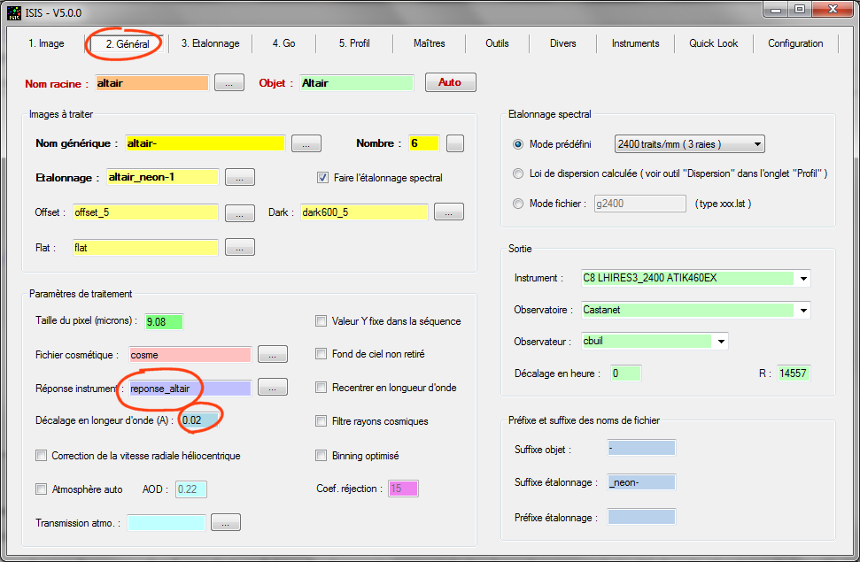
We provides the name of the instrumental response calculated (before ISIS was able to treat the spectrum, but by the approximation of a perfectly flat response). We took the opportunity to tell more in our ISIS spectrum has a spectral calibration error of 0.02 A when processes with the current settings. Remember, we found this value by comparison with the expected position of the H2O telluric lines.
Directly open the "Go" tab without using the "Calibration" tab, because all other parameters being unchanged, then press "Go" button:
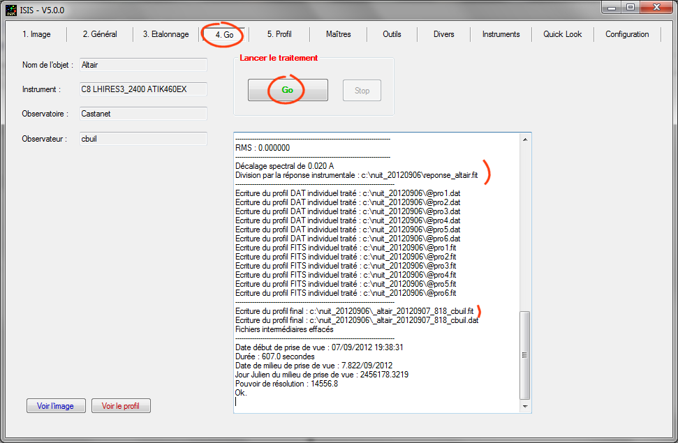
Everything seems like it happened in our first processing. However, there are nuances and ISIS tells you in the output info window, giving information about processing (informatiothat you learn to decode as and as you take hold of the software). Note that the spectral shift of 0.02 angstrom is taken into account, and the division by the instrumental response. View the final profile (either by clicking on the "Display profile" button or by opening the "Profile" tab, then clicking the "Display" button:
It's OK for Altair star, you can go to the next object !
Tip: a good reflex is to compare your processed spectrum to that achieved by a third party. Here we make a comparison with a spectrum of Altair made with the Elodie spectrograph, but now without removing the telluric lines. From the "Profile" tab, press the "Compare" button. The window that opens is one of most important ISIS tools. You use it often. It can display on the same graph two distincts spectra for comparison. Here we have selected the file "elodie_altair.dat" located in the ISIS database directory (here, c: \ isis_data). Note that files coming from Elodie are stored in .dat file format (simple ASCII list of numbers in two columns). You must precise this in the dialog box "Compare two spectra". Now click on the red "Compare" "button:
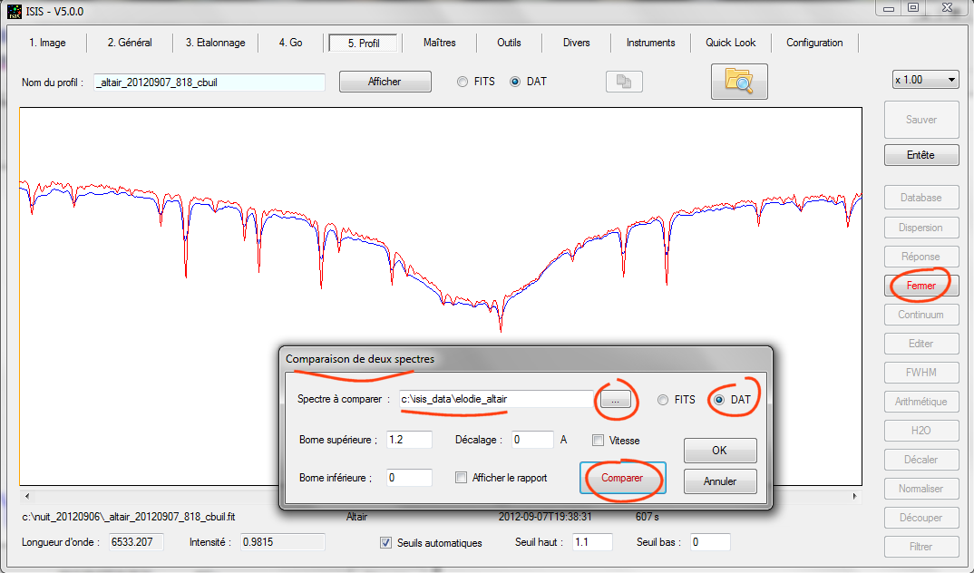
The result is spectacular. Ok, Elodie spectrum is twice spectrally resolved compared to our Lhires III spectrum , but there is very good superposition of
telluric lines, which mean that the spectral calibration is excellent (do not mind the Halpha lines because presence of the spectral shift due to the Earth heliocentric velocity). The continuum is also very well restored through the processing treatment. All parameters are green.
It is therefore now possible to process very fast and safe way all your spectra. ISIS becomes a production tool particularly effective. To feel good,
we going to completely process the sequence of spectra for the star 28 Tau, taken the same night...
4. Routine processing
From the "Image" tab display the first image of the sequence to remind this:
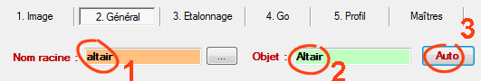
Click "General" button (not the tab item). The "General" tab opens. It is already pre-filled. Your only job is to specify the catalog name for the object ("28 Tau").
We also set to zero spectral shift, nothing in fact indicates that our spectrum is not calibrated correctly at the end (to stunned, ISIS knows
detect that you deal with a new spectrum and if you do not have set to zero this field , it alerts you and asking for confirmation).
Tip: the step of displaying the image may be skipped if you're the kind of hurry. To do this, at the top of the "General" tab, enter the name of your root sequence, the name of the object, and finally, press "Auto" button:
This is optional, but made a quick tour through the "Calibration" tab. In this way, ISIS automatically updates the Y-value of the coordinate of the spectrum trace. You can also do a visual inspection of the binning area (in particular verify that the two blue lines completely cover the width of your spectrum - an important prerequisite for a good spectral photometry in the final):
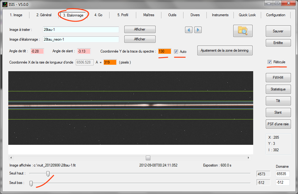
Open "Go" tab, the click on "Go" button:
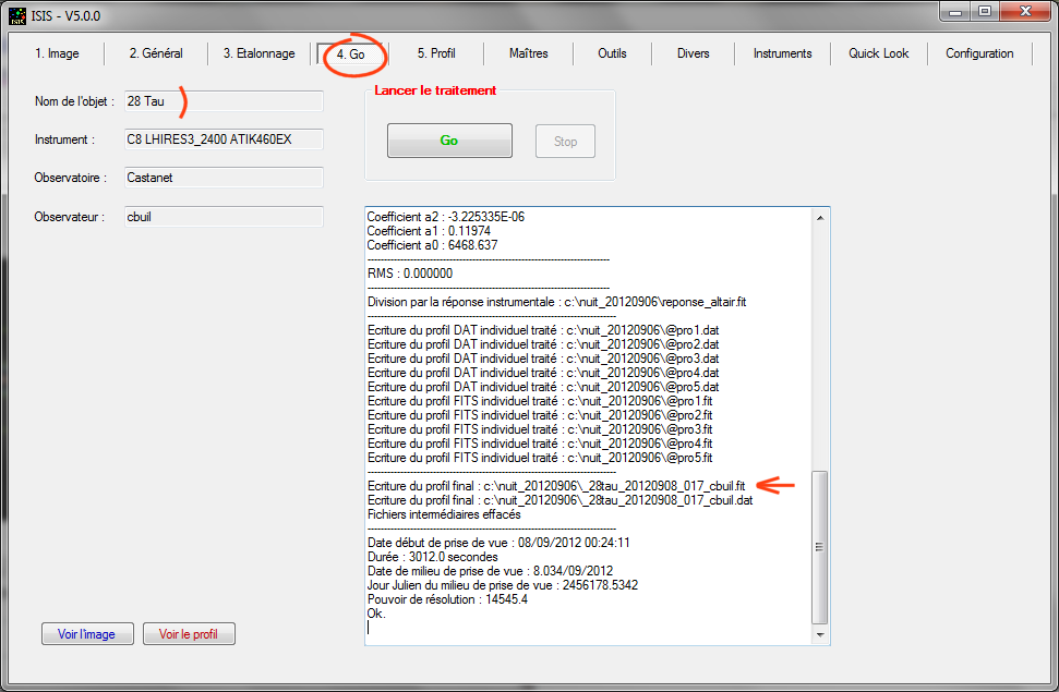
The processing is completed, display the result:
You can process to the next star, and so on.
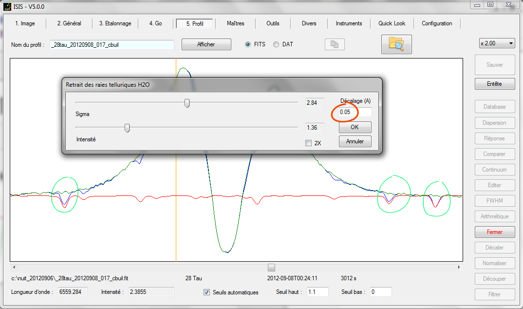
Tip: remember to check the quality of your spectral calibration for excellence. A simple way is to display on your stellar spectrum the theoretical spectrum of water vapor if you work around Halpha line. Click "H2O", adjust the sliders (note that the value of "Sigma" parameter in particular is the same as that adopted in the Altair processingr):
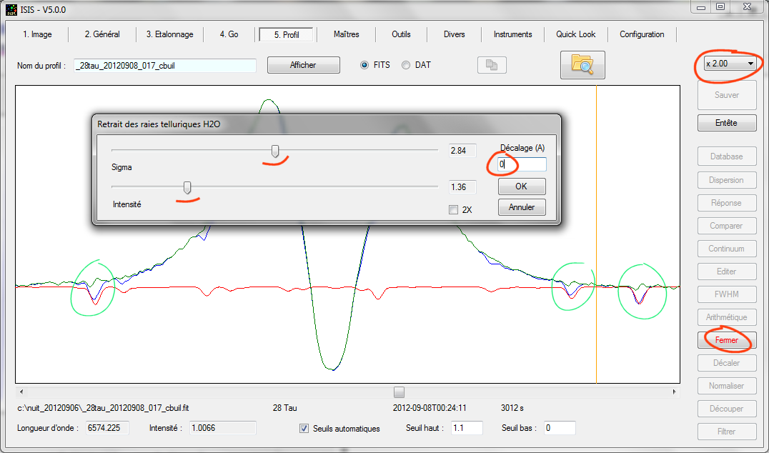
Contrary to appearances, the calibration is not as perfect as this. Look telluric lines residue in the green line profile. Obviously, our 28 tau spectrum has a slight lack of calibration. Although subtle, but significant. By trial and error you will soon see that the shift is 0.05 A (note that you can also find negative values, depending of the sign of calibration error):
Exit the tool by clicking "Cancel" (or "OK" if you really want to remove telluric lines from your stellar profile, which can be useful for some studies). My recommendation to handle this situation is to raise the value of the spectral shift, and report in the "General" tab:
Then resume processing from the "Go" tab, which is very fast:
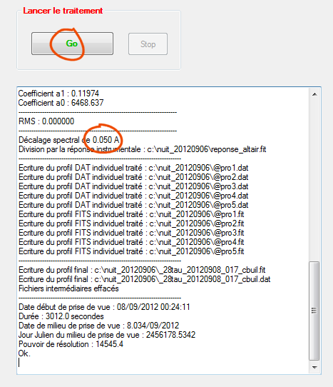
The resultat is now perfect.
5. Complements
Some recommendations and tips now.
Rather than a simple addition along column axis, ISIS can use an optimal binning strategy for compute the spectral profile from the image. The idea is to give more importance to the pixels of the image the most strongly illuminated. This method is almost universally proposed in all institutional spectra processing software (MIDAS, IRAF, ...). To work in this mode, selected "Optimal binning" from the "General" tab:
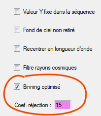
The associated rejection coefficient fixed force for removal of cosmic rays. The value 15 is a good choice in general. This optimized binning method is so powerful and effective (especially if you take spectra of very faint object) that it is recommended to always select ISIS the option (the signal to noise ation will be improved).
ISIS offers a complementary tool to eliminate cosmic rays. The method used is effective, but also quite aggressive:
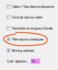
Generally there will be no problems with the Lhires IIII spectra from Lhires III because they are well sampled by the pixels detector (about 3 pixels and more in the FWHM). So, yes, with Lhires III, you can check this option (control the difference with and without this option in the final profile). However, it must be much more careful with LISA spectra or sometimes spectra acquired with simple Star Analyser grating. These spectra are often so thin that the filter can alter the real parts confusing them with cosmic rays. Therefore caution, and with these data, avoiding using such a filter, if possible.
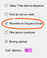
With "Wavelength registration" selected ISIS checks for each spectrum in a series a relative spectral shift and realizes the operation for register the individual profiles to the first of the sequence. In this simple button that hides a correlation method and a few refinements that make this feature one of the most powerful tools of ISIS (I used these algorithms to measure exoplanets radial velocity by using amateurs instrument). Note, however, the accuracy of the result is directly related to the spectral content (if the spectrum shows no lines, the technique fails of course) or noise in the data. Take the example of 28 Tau. First do:
Then start processing from "Go" tab. Here's what returns ISIS:
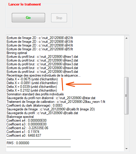
It is learned that the second spectrum of the sequence (28tau-2) is shifted by -0.0675 pixel (remember the pixel size is 9.08 microns, so the linear shift represent -0.0675 x 9.08 = -0.6 micron) compared to the first spectrum of the sequence along the spectral axis. This discrepancy reaches up to 0.21 pixels for the final spectra acquired. ISIS in the background work to recenter these spectra with the values measured. However, here the spectral shift is very small and the technique used give not a real gain in this case (gain is expected to improve the spectral resolution and lineshape better mastered). However, the situation may be much more difficult. To see this, here the diagnosctic (exact) of spectral shift when observing a faint star on a long-lime (AZ Cas):
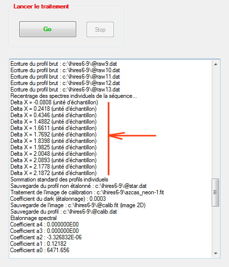
The exposure time for each spectrum of the sequence is 600 seconds. The total observation duration is more than two hours. The spectrograph take an hour for mechanically stabilize, but the drift is in fact almost continuously. The spectral shift between the beginning and the end of the observation is of the order of 2 pixels, a value close to the spectral resolution element. This results correspond to a calibration error and spectral line broadening that can be corrected if the option "Wavelength registration" is checked. Attention, AZ Case is a type M star, with numerous lines in the observed spectrum - the result may not be as accurate with a hot star - as always, be sure to controm the action of your decisions - all is not so simple! So how to check? During processing ISIS write on the working folder many intermediate files to diagnose potential problems. This is particularly true of the sequence files "@proxxx.fit". This profile correspond to spectra extracted from individual input images. ISIS construct the final profile by addition the containt "@pro" files:
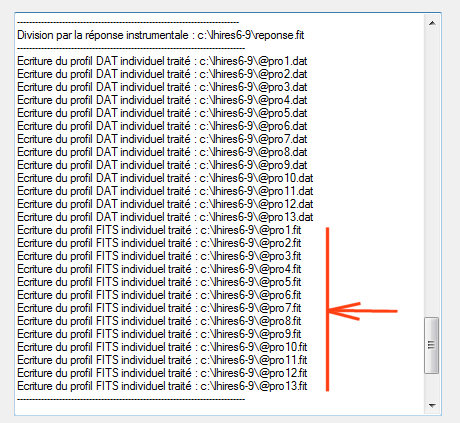
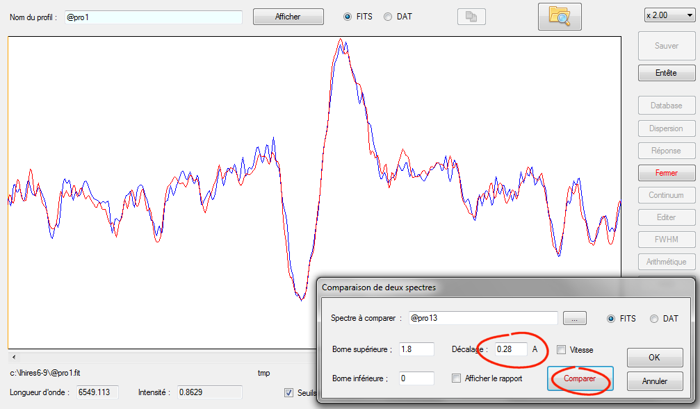
Display these individual profiles from the "Profile" tab and compare two by two with the "Compare" tool (eg the first and last sequence profiles). Warning, these intermediate files are deleted automatically at the and of processing if you command this action (see "Erase automaticaly intermediates file" in the "Settings" tab). For example:
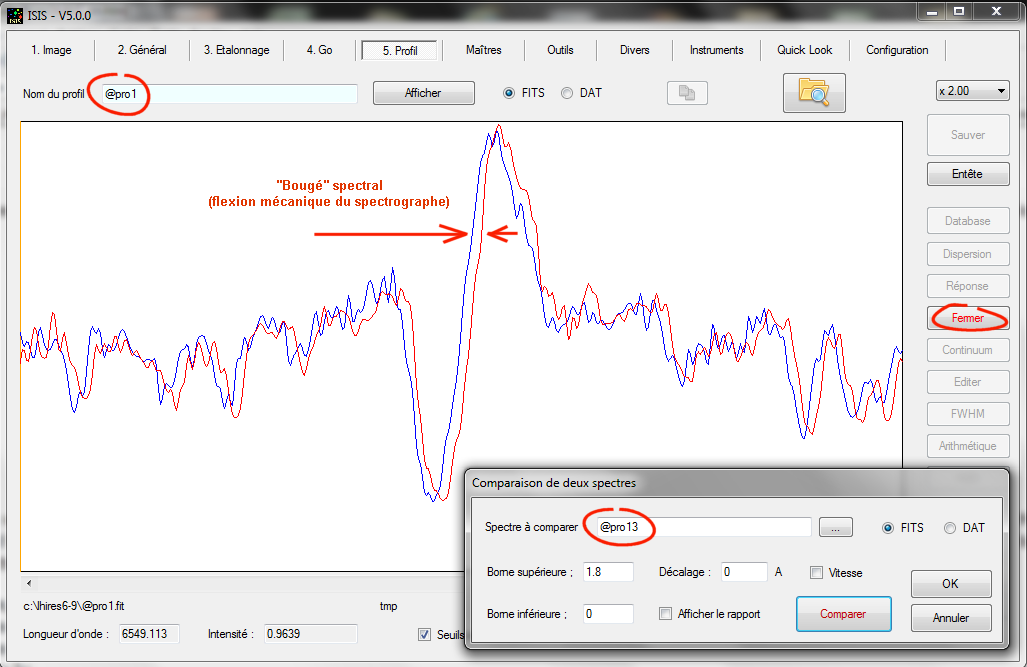
Note: You can manually recenter the spectra, but the operation is fastidious for large sequences ("Wavelength registration" option is more automatic !). For example here we find a spectral shift of 0.28 A by a simple visual inspection:
Recommandation for spectra acquisition: In situation of wavelength drift with a long duration Lhires III sequences, an intuitive solution is to take a spectrum of neon lamp at the beginning of the sequence (azcsas_neon-1, for example), and then a spectrum of neon lamp at the end of the sequence (azcas_neon-2), and so, calculate the average of both:
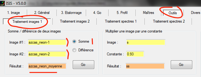
Indeed, one idea is to use the image azcas_neon_moyenne (= azcas_neon-1 + azcas_neon-2, equivalent to an average) to process the spectra by this way:
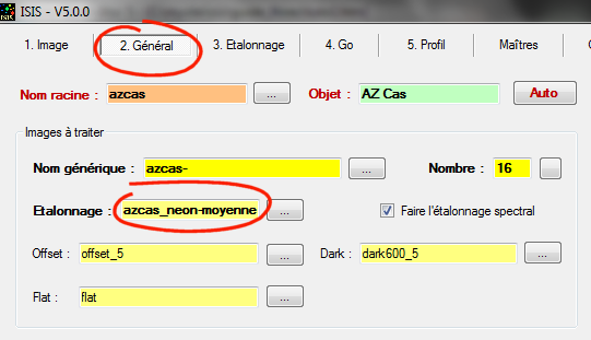
This works, no problem: we minimize the calibration error. But beware. ISIS evaluate spectral resolution from the given calibration image (mean FWHM of neon lines used for spectral calibration), and of course the result is now incorrect - middle image is somewhat blurry. More serious is the loss of spectral resolution on the final spectrum. The best protocol to make during acquisition is propably:
azcas_neon-1
azcas-1
azcas-2
azcas-3
...
...
azcas-16
azcas_neon-2
Then, use azcas_neon-1 as a reference because it is temporally located near the first image of the sequence (azcas-1), then, if possible, select the option "Wavelength registration" under ISIS (reminder, the software register relative to the first frame of the sequence). The image azcas_neon-2 serves as a control data.
Another point. Suppose you want to extract the spectral profile of neon lamp. The exercise is important because it indicates method for extract spectrum of extended objets, occupying a large height on the entrance slit of the spectrograph (nebulae, comets, ...). Here, how to complete the "General" tab to solve this problem:
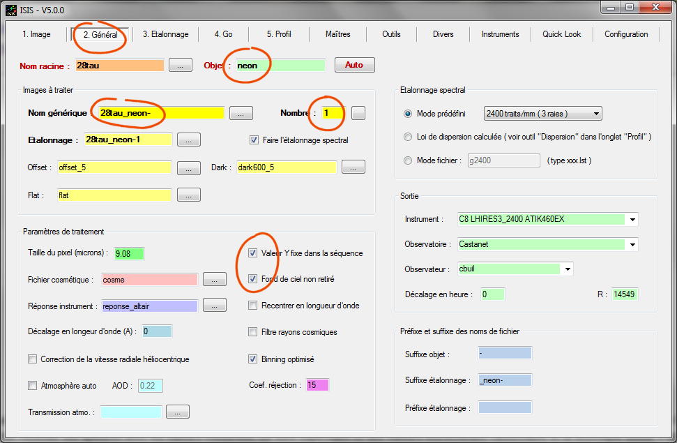
For the name of the object, we adopt "neon" - why not!
Note the generic name provided: "28tau_neon-". This is ISIS will add the index number to build the full file name. Note that we have only a single image. Our neon spectrum is calibrated here with itself, that is why we adopt "28tau_neon_1" for the input calibration image name.
Tip: If you process only a single image and that it has no index number, you can enter the name in the "generic name" but you must specify a number of frames equal to zero. In this case, the indexing system is not activated. For example, the processing will work perfectly in our example if you specify a generic name like "28tau_neon-1" and a number of frames equal to 0 (ISIS does not then add an index number to the generic name).
I also selected the option "fixed Y value for sequence." This prevents ISIS to perform shift on 2D images along the vertical axis for register individual spectra (needed for internal operations). The operation has no meaning when dealing with extended object spectra (non-pointual objet) and can even be harmful.
I also enabled the "sky not removed." In your actual situation, if ISIS removes the sky background around the target object (neon lines), the spectral lines are
simply disappear, which is not the goal. So we active a non removal sky background mode. The rest is unchanged in this tab.
Then open "Calibration" tab
I unchecked the option "Auto" for the Y coordinate, I entered the value by hand (or by double-clicking in the image) - towards the center of the lines. I also expanded the binning area via "Binning adjsutemnt" dialog box, the idea here is to have a generous signal and thus a spectral profile of quality (not to exaggerate the binning height because the lines are slightly curved and it would degrade the spectral resolution). There is nothing else to do in this tab.
Run the process from the tab "Go", then check the result:
We have obtained Lhires III spectrograph neon lamp spectra.
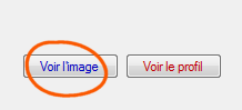
About this processing, from "Go" tab, press the button "Display image":
you can examine the 2D neon image geometrically corrected (operation made above the binning):
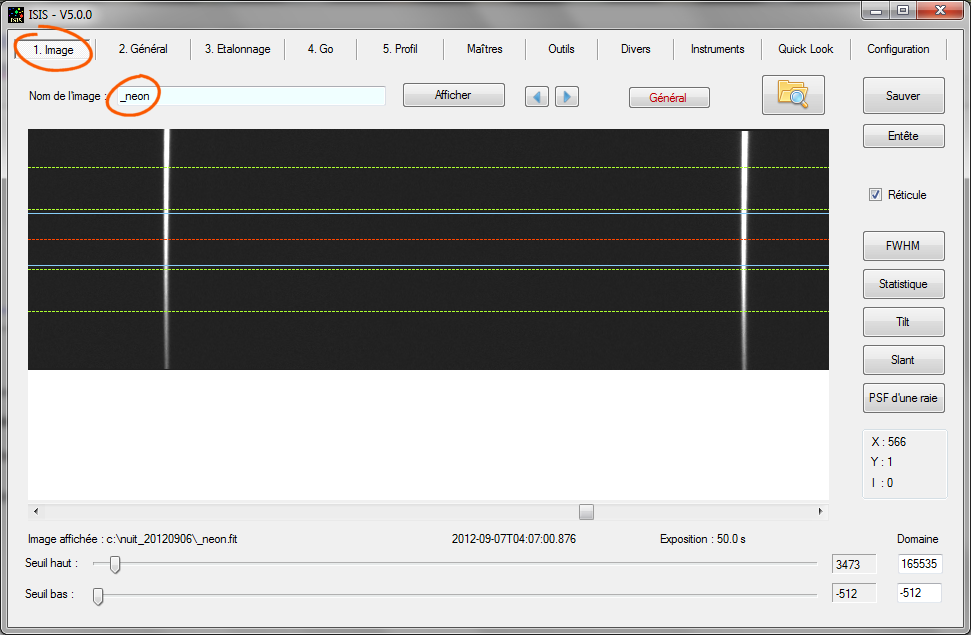
If you process a sequence of stellar spectra, this control image also contains the sum of all individual spectra.
After this excursion in the domain of extended spectra processing we reprocess now stellar spectra, so think especially to uncheck the options "Fxed Y value for sequence" and "Sky not removed" and adjust the binning zone value if necessary. Do it right away to avoid nasty surprises!
If you are using a spectrograph Lhires III in particular, it is possible to increase the spectral resolution slightly if you select the "Spline" interpolation method from the "Settings" tab:
In this way, internal processing less smoothing the data. But, if your spectra are at the limit of sub-sampling as with LISA spectrograph instrumental in some configurations, the interpolation "Spline" may cause artifacts in the final profile. This is the reason for which the choice of the interpolator is available in ISIS.
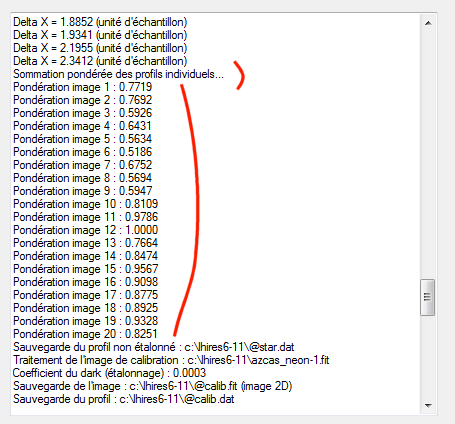
Note also that you have the choice of summation of the individual spectra in a sequence. The "Standard" mode is a simple sum. The "Weighted" option activates a procedure that gives more weight to the most intense spectra in a sequence. The option is optimal for process a sequence where remlative intensities of individual spectral is very different. Below is an example where there is a large variation in weight, indicating a cloud passage during the observation (for the final spectrum, contribution of spectrum # 6 will be 50% less then spectrum # 12):
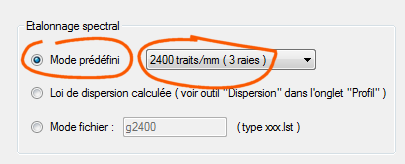
One important note now concerning mode available for wavelength calibration. We previously used a mode called "Predefined mode", expected for process Lhires III spectra around the Halpha, while the spectrograph is equipped with 2400 lines / mm grating. A very restrictive and specific choice:
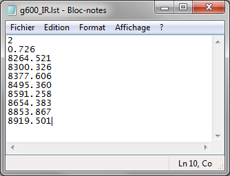
But what if your spectrograph uses a g600 lines/mm grating or if you are targeting the ultraviolet or infrared regions of the spectrum?
The solution is the "File mode":
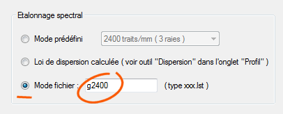
By selecting this mode, you specify a file name as text (ASCII format, editable with notepad application for example). In the example, this file is named "g2400" (extension. lst is automatically added by ISIS). The file must be located in the working directory, or better, in the CALIB subdirectory if you have had the good idea to create one. You can adopt a different name (here, the "g" stands for "grating" and "2400" indicates the number of grooves per millimetee, a way of recognize the content, because you can have a collection of calibration files describing several instrumental configurations). Here, the contents of g2400.lst in our example:
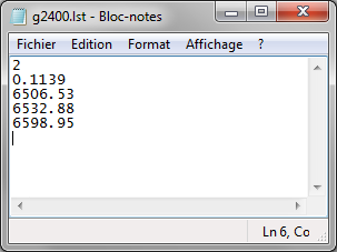
We immediately recognize the wavelengths of three neon lines that we use from the beginning (6506.53, 6532.88, 6598.95) - a wavalength by line in the file.
The first line of this file is the degree of the polynomial adopted for dispersion equation. A high degree can fit better dispersion of nonlinearity. But it is not always happy to work with a strong degree. This gain in accuracy may be an illusion. This is the case in especially if your calibration lines are all concentrated in the center of the image. In this case, the calibration of the edges of the spectrum may be catastrophic (a polynomial dispersion is made to interpolate, not extrapolate not). Anyway, if you have n lines of calibration, the maximum possible degree is n-1.
In our example we have only 3 lines, and quite logically, the degree of dispersion equation is 2 - a good choice here. The maximum degree is accepted by ISIS is 4.
The second line contains the dispersion (reciprocal) average in angstroms per pixel. In the example we have adopted 0.1139 A / pixel. This value is easy to find: from the "Image" tab measure the gap distance in pixels between two known lines in the spectrum of the calibration lamp. The desired value is then equal to (difference in wavelength between the two lines) / (gap in pixels between the two pixel lines). There is no need to search high accuracy, it is right here a medium dispersion medium.
Finally found a list of lines present in calibration lamp, if possible bright, unsatured and well isolated. It can be an unlimited number. ISIS will automatically identify the lines in the spectrum.
Here's how it use the calibration file mode. First, as we have seen, from the "General" tab, choose mode "File mode", and then specify the file name list containing the parameters. The other difference is in the "Calibration" tab. You must implicitly provide the wavelength of the reference line for where the X coordinate is measured:
You can select any line (but if possible well exposed in the calibration image). Everything else is similar to the standard procedure described in this guide. If you made "Go" in this situation, you'll find exactly the same result as the calibration mode preset.
The calibration from a file of lines gives considerable flexibility. This is what makes the "universal" character of ISIS: you can process virtually all spectra with the software, regardless of the source. For example, here is the lines file list that I use to calibrate spectra from a spectrograph Lhires III equipped with a 600 lines/mm grating set around the CaII infrared triplet (see details here):