Processing of  Star Analyser spectra
Translated by Robin Leadbeater

Version en français

Pleiades cluster observed with the Star Analyser 100 on the front of a 100mm telephoto lens. The recording was made using a digital camera 
 

For practical purposes, we will process a sequence of seven images taken in succession with a Star Analyser 100 placed a few inches in front of the detector. The star is Delta  Cas. The telescope is a C11 and camera model QSI532.  The exposure time is 1 second.

Figure 1 shows an example  of an image in the sequence.  (reduced in size)

The ISIS wizard for processing SA spectra performs a crucial operation when it comes to treating  SA spectra : geometric transformation, making the dispersion axis horizontal, with wavelength increasing from left to right (see Figure 2). If we treat a sequence of images, ISIS also aligns the spectra on top of each other, automatically adding them.  The wizard also automatically removes the sky background and extracts a raw (uncalibrated) spectral profile. 

From that point , the ISIS calibration tools can be used to complete the treatment.

Figure 1. Raw spectrum of Delta Cas.

Figure 2. Geometric transformation done by  ISIS.
 

Step 1. Measurement of the zero order position

Open the tab "View image" and view the  first image to be processed (first image in the Delta Cas series - these images were saved at the time of acquisition with the generic name "DCAS-").  Find the X and Y coordinates of the zero order image using the mouse pointer, or better, using the FWHM tool  (Figure 3).

Note   The  coordinates here are X = 579.7 and Y=714.5 (high precision is not imperative, these pixel values are sufficient).

Then measure, still in pixel coordinates, the position of a  point in the spectrum.Use the mouse to point to it (Figure 4). The position is not critical provided it is on the spectrum line. Here we have used X = 581, Y = 239.

 

Figure 3. Coordoninates of the zero order image.



Figure 4. Coordinates of a point in the spectrum.

Step 2. Measuring the orientation of the   spectrum

 Open the tab "Star Analyser."

Go to the section "Evaluation of the orientation". Note that the fields X0 and Y0 are already pre-filled. This was done in the background when you called the function FWHM in the previous step. This reduces the risk of  errors from retyping the numbers. 

Fill in the fields for  the X and Y coordinates of the point on the spectrum  with those selected in step 1.

Click "Go".  ISIS returns the orientation of the spectrum compared to the horizontal axis (here -89.84 °) - see Figure 5. Note that the "Direction of the spectrum" is automatically filled in after the calculation.

Figures 6 clarifies the sign convention for the angles.

Figure 5. Calculation of the spectrum angle.



Figure 6. sign convention.

 

Step 3.  Assigning the required position of the zero order in the rotated image

When  ISIS makes the geometric transformation, it does not just rotate around the zero point.  It can also move laterally (ie make a translation).

This possibility is very useful because the spectrum can be very accurately adjusted to the chosen location. In our example we choose the coordinates of the origin = 200 X, Y = 300 (see Figure 7).

This choice may seem  somewhat arbitrary, but it ensures that the processed spectrum will never overlap the edge of the image.

These same coordinates can be adopted routinely for all your spectra, which will position them in the same place in all the processed 2D images.  This is useful for comparisons, to demonstrate the diversity of spectra, educational purposes, etc.

This rotation/translation function is very flexible and can also be used to solve other difficult problems. You will probably find other uses for it.

Figure 7. Final coordinates for the zero order image (We have chosen X = 200, Y = 300).



Figure 8. Assigning the final coordinates for the zero order .
 

Step 4. Finalising the input parameters 

We will process a sequence of 7 images of delta Cas.  At the time of the acquisition we gave the images a short generic name, here, "DCAS-" (The image files are called DCAS-1.fit, DCAS-2.fit, DCAS-3.fit,. .., DCAS-7.fit).

Enter the generic name and the number of images in the appropriate fields on the tab "Star Analyser"  (see Figure 9).

Finally, you should specify a meaningful name for the object, allowing you to better manage your image files for further treatment.

Figure 9. Use the Official" name of the object and generic images to be processed (that name will be traceable to the database of object names in CDS Starsbourg). Absolutely avoid exotic names, such Rasalhague, Sadr, and so on.  For a scientific database, a record with the HD number (HD159561) will always be much more effective . You will also be taken much more seriously by the astronomical community as a whole   

Step 5. Running  the processing and analysis

Now click on the button "Go". The treatment only takes a few seconds (Figure 10).

ISIS performs the complex operations for you. In particular, the individual 2D spectra are perfectly aligned relative to each other, although at the time of observation the telescope moved between the exposure (to some extent it corrects tracking errors).

In this step ISIS generated many intermediate files that allow you to have complete control of the processing .

However, the most immediately interesting product is the calculated spectral profile.  It is saved with two names: @ raw.dat and ObjetName_raw.dat. The contents of these files are identical (in the second form, the name of the output file is "delta cas_raw.dat" a little long to handle, hence the existence of a more compact file name "@ raw.dat "to help you).

 If you click on "View profile", the spectral profile of our star is immediately displayed (see Figure 11).

Among the intermediate files, note that the file   @@.fit Contains the composite image made ​​from all spectra before the removal of the sky background and the image @ @ @. fit (or NomObjet_2D.FIT) is the composite image after removing the sky background.  As always, these images can be viewed from the tab "View image".

The parameters used for binning the 2D spectrum to extract the spectral profile and the calculation area for calculating the sky background are fixed as always in ISIS from the tab "Configuration". This issue will be discussed in detail now.

Figure 12 shows example image @ @. fit of Delta Cas after the addition of the individual images.  It is displayed with high contrast.  Remember that in the picture "@ @", the sky background is not removed.  The binning zones for calculation of the sky background characteristics are shown,  but depending on the situation, you will need to   change their width and position (eg to exclude a bright object from the calculation area).  fig 13 shows the part of the tab "Configuration" which is used to configure the zones.

Figure 14 displays the processed image after removing the sky background (image @ @ @. Fit).  Remember it is always possible to visualize the areas used to calculate the sky background by selecting the "Setup" tab (check button "Show").

Tip:  To see residual background, do not hesitate to set negative  minimum value for the intensity scale (eg -200 as shown in Figure 14).

Figure 15 presents a typical example where the calculation area of the sky is too close to the spectrum of the spectrum of the object studied. Part of the sky background is in fact the signal from the spectrum which skews the calculation. (This is seen as high negative values in the sky background after subtraction when it should be close to zero).

Figure 10. Starting the treatment.

Figure 11. The raw spectrum. Note that the horizontal axisis scaled in pixel numbers. the spectrum is not yet calibrated in wavelength.
 


Figure 12. Bining zones for calculating the sky background.

Figure 13. Adjusting the sky background binning zones.

Figure 14 2D image of the Delta Cas spectrum after removal of the sky background. (intermediate image @@@).

 

 Figure 15. Example of incorrect removal of the sky background.
 

Treatment using   "Expert" mode

 If you click  "Expert" in  "Star Analyser", the processing performed is more accurate and rigorous. ISIS then performs a comprehensive pre-treatment (see Figure 16).

You must provide an offset image, a dark signal image(corresponding to the exposure time for images to be processed), and a flat-field image. Optionally, you can also provide a file containing list of points to erase cosmetics, and even filter out cosmic rays (note: if this option is selected, the processing time is greatly increased ).

It is very strongly advised to start using the "Expert" mode as soon as possible. This will benefit all your spectra.

As an illustration, Fig 17 shows a flat field  of the twilight sky taken using the Star Analyser (note  the significant vignetting in the corners of the field. It is is job of the Expert treatment  mode to eliminate these defects in the processed image).

 
Figure 16. Expert mode.

Figure 17. Flat-field taken with a Star Analyser (note the presence of dust in the optics and the vignetting).
 

Step  6. Wavelength calibration

Delta Cas is type A5III type star, with a series of hydrogen lines suitable for a spectral calibration clearly seen.  We also have the line from molecular oxygen in the infrared (7605 A) and the zero-order spectrum, which can be likened to an emission line of wavelength  zero Angstrom. Figure 18 shows the position of these lines and their wavelengths.

Open the tab "View Profile" and then click "dispersion".

We will first evaluate the position of the zero-order pixel along the spectrum.

Note: the order of entry of spectral lines in the dialog "dispersion" does not influence the final result.

Since the zero order appears as an emission line, select this option at the top of the dialog box (see Figure 19). Double click to select the two sides of the "line".  ISIS finds the pixel position X = 210,010. Specify 0 Angstrom for the  wavelength of this "line" (a bit strange, but useful anyway).

We will now select the line Hdelta (Figure 20). Warning, this is an absorption line, so this option is selected in advance. ISIS finds the position X = 449,805. Enter the corresponding wavelength of this line in the dialog box "Calculation of spectral dispersion."

Continue in the same way for all lines of your choice (the number is free, up to a maximum of 12 ).

In our example we are going up to the O2 line at 7605 A. There is no problem if you're wrong, you can always re-select the line that is the problem in the list.

Most of the work is done. Whew!

Note: you can calibrate your spectrum with only two lines, but the result will be much less accurate.  As in an a ideal world, the extra effort pays off.

Choose a polynomial of order 3, then click the "Calculation of the polynomial" at the top of the dialog box (Figure 22). 

The  polynomial coefficients of the dispersion are returned. For example, the coefficient A1 gives the average dispersion.  Here it is 23 A / pixel.

The residual error of the calibration is 7 A, which is satisfactory for this type of optical configuration.

Without closing the box, to calculate the spectral dispersion, click "Calibrate".  The calculated coefficients are applied to the  current raw profile displayed. Now close the dialog.

Note: ISIS prevents you from running "Calibrate" a second time.  This is normal because your  spectrum is now already in calibrated in wavelength.

Your wavalength calibrated spectrum is now displayed (Figure 23). If you move the cursor in the trace, you'll see that now it shows wavelengths.

Figure 18. Identification of the spectra lines used for wavelength calibration for a star of type A or B.


 

Figure 19. Selection of the first line (zero order)

Figure 20. Selection of the second line (Hdelta). Atention, this is an absorption line. You must tell ISIS this first!

Figure 21. Selection of the last line in our  sequence (The O2 band from the Earth's atmosphere)

Figure 22. Calculation of the spectra dispersion.



Figure 23.The wavelength calibrated spectrum.
 

More... 

At this point you can of course save your processed spectrum in DAT  or FITS format. To create a BeSS compliant FITS-, first generate a DAT file (TMP.DAT example - see Figure 24), then a FITS file from the tab DAT-> BeSS (see Figure 25 ).

In fact, before publishing your spectrum, it is a good idea  to eliminate the Astrophysically meaningless parts of the profile  (zero order, for example) and the problematic regions (for example, over the wavelength of 8000 A where the overlap between the order 1 and order 2 cause a measurement bias making an incorrect measurement in  the infrared part of spectrum. A good idea is to keep only the  actually useful region  using the tool "Cut" from the tab "View Profile" (see Figure 26).

Figure 24. Save the spectrum in the DAT file format.



Figure 25.An example of creating a FITS file compatible with the BsSS database from the DAT file. Note that we have supplied time of observation as a fractional day.
 


Figure 26. Cropping the useful part of the spectrum.
 

Even further...

Even though  our spectrum is  wavelength calibrated correctly, it is not calibrated radiometrically. The general shape of the profile intensity is largely affected by the instrumental response, not the actual spectral distribution of flux received from the star. We find the true spectral distribution by dividing the current profile by the profile of the instrumental response.

It is perfectly possible to exploit the functions of the "General" tab to evaluate the instrumental response, and then apply the correction to our spectrum. The fact that the latter is of type A facilitates the operation.The description of these operations is beyond the scope of this tutorial.  The procedure is widely described in several other places in the ISIS documentation  (see especially the pages devoted to the treatment of spectra LHIRES III and LISA).

I will just give here the procedure to properly complete the data entry  needed in "General" tab.

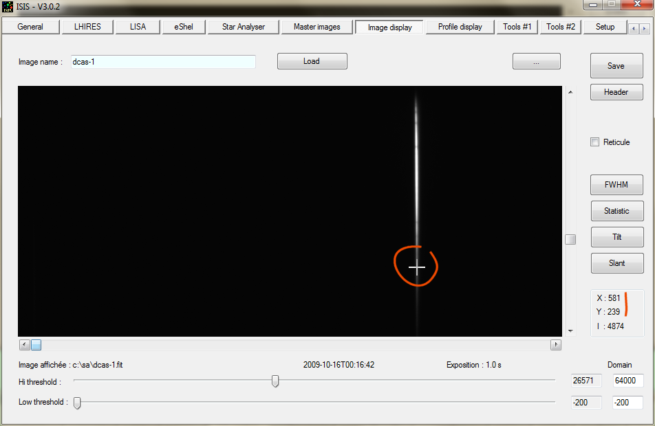
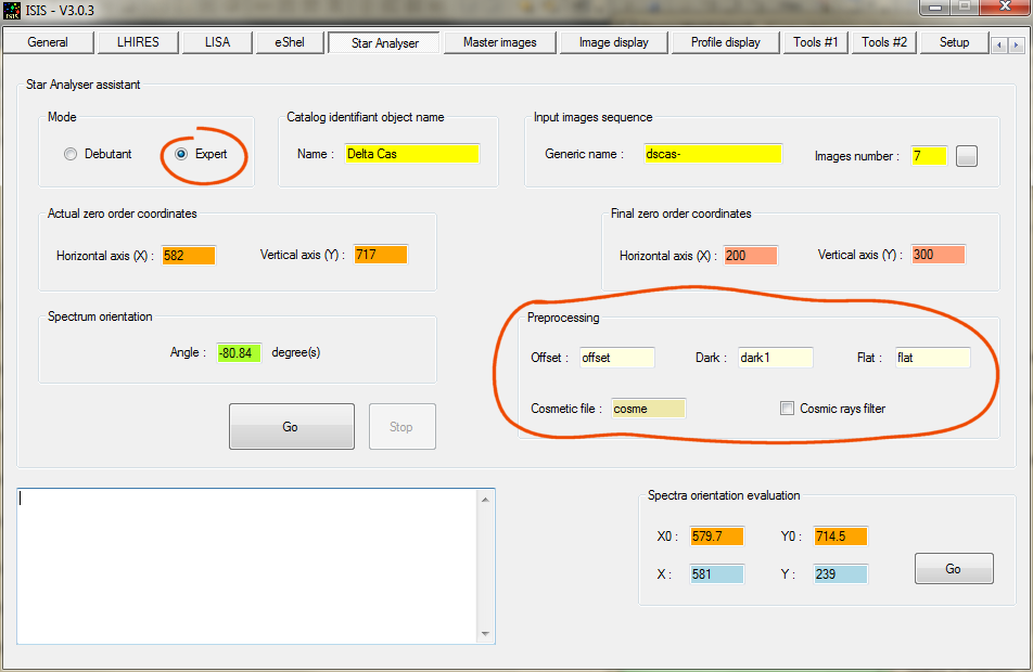
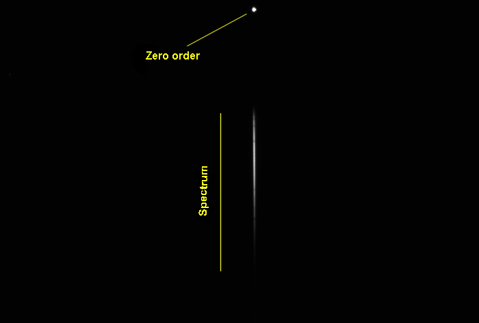
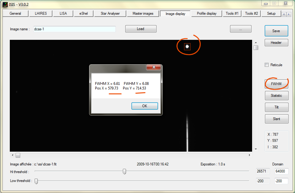
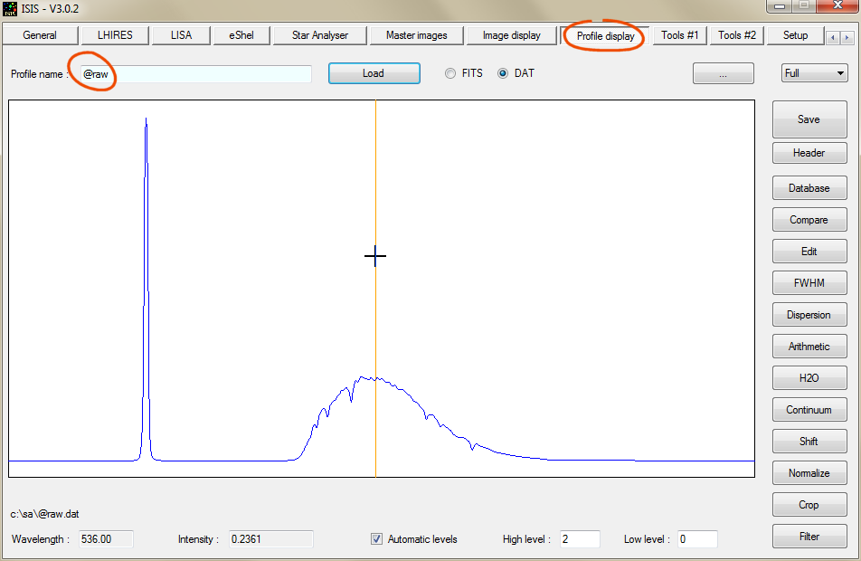
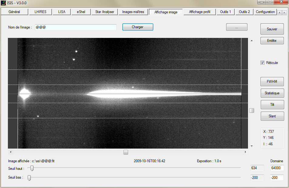
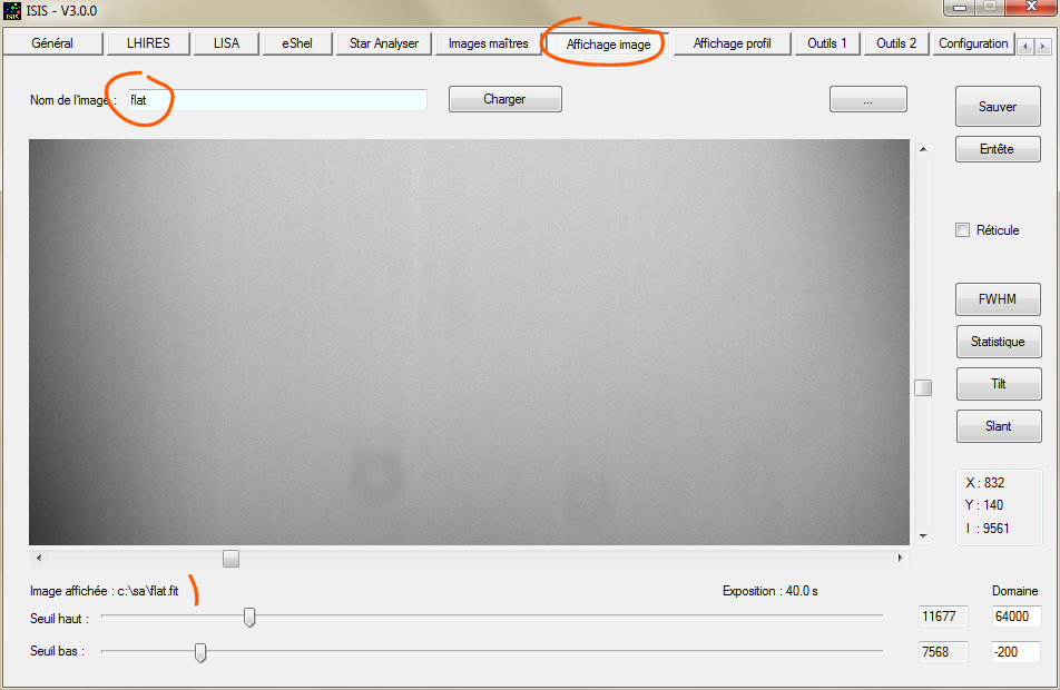
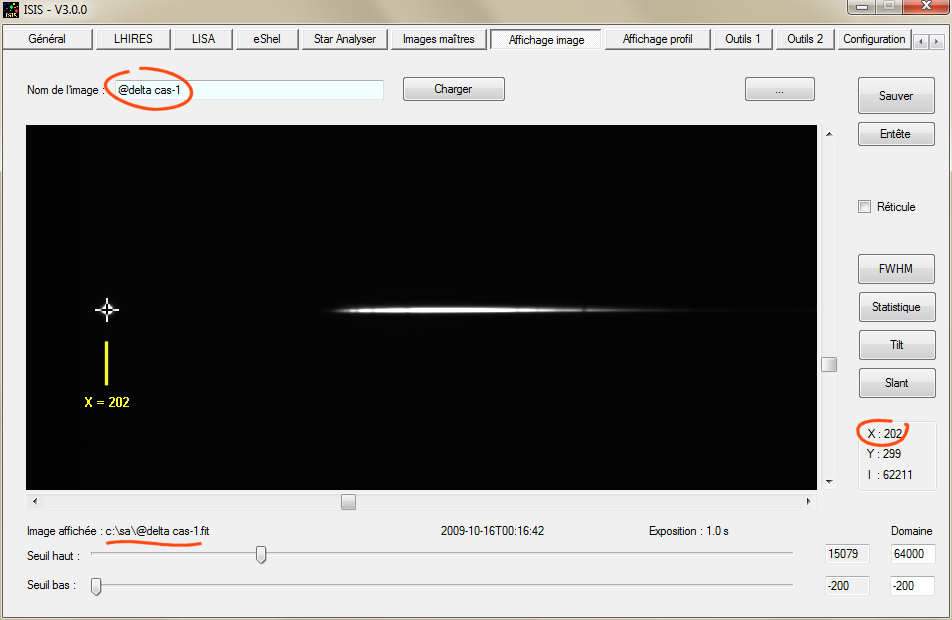
We must first note that the wizard "Star Analyzer"  produces 7 preprocessed 2D images  (if you are in expert mode, which is recommended).  These images are perfectly corrected  geometrically (the spectrum is horizontal).  They correspond to the seven initial raw images.  Their names in the working directory are @ObjetName-xxx.fit. For example, Figure 27 shows the visualization of the first pre-processed image of the sequence. We mark the horizontal position of the zero order, which not surprisingly,  is around  X = 200.

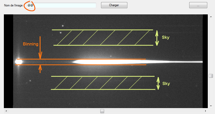
Note that the sky background is not removed from the 2D spectra of this sequence.

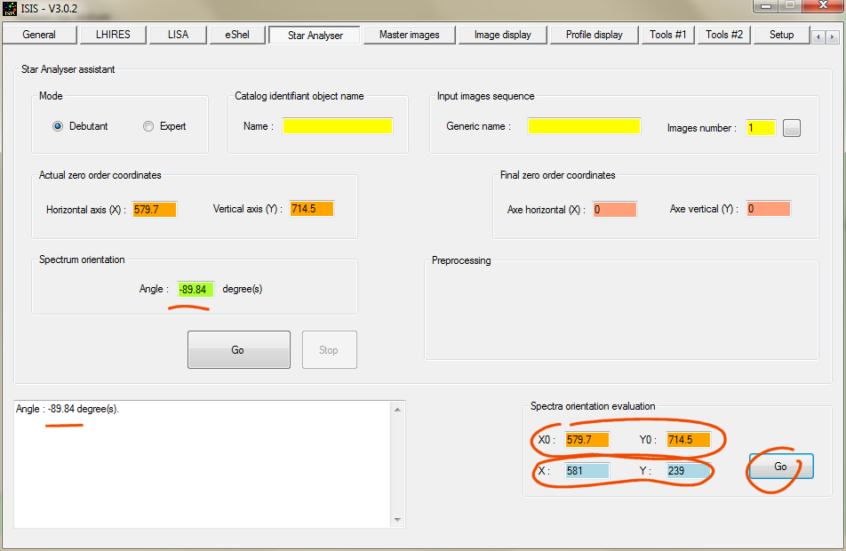
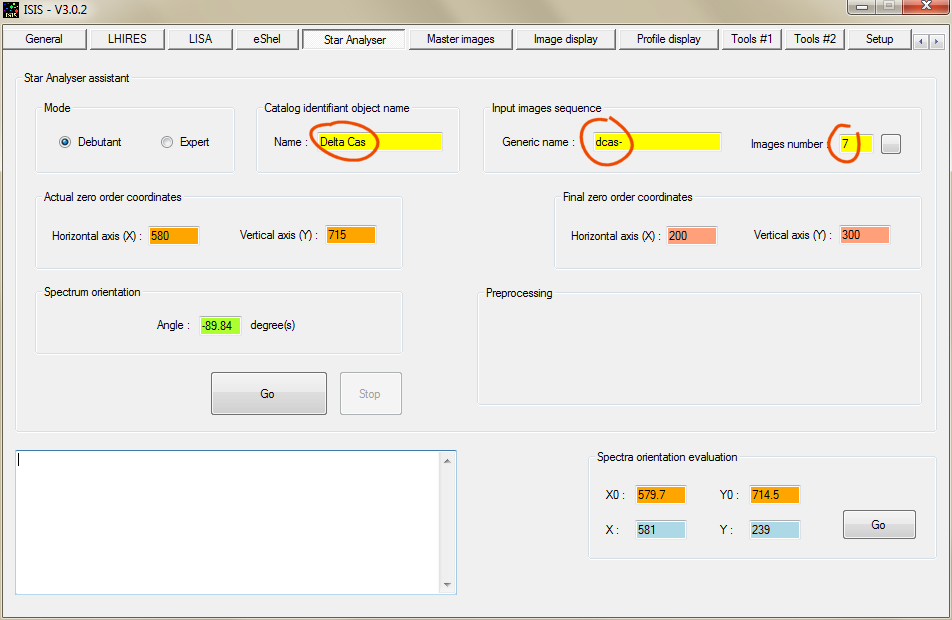
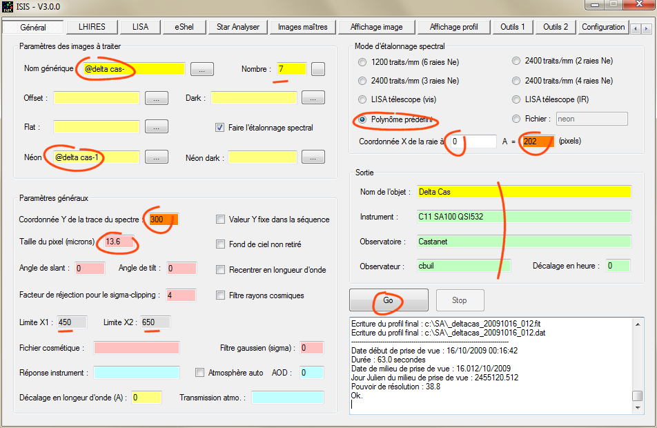
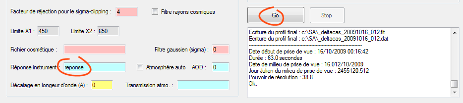
Then open the "General" tab and fill it out as shown in Figure 28.

Provide the generic name for images to be processed (here @ delta Cas) and the number of images in the sequence (here 7).

The pretreatment is assumed to have been achieved by the assistant "Star Analyser" you do not have to do it again at the "General" tab.  To indicate this fact to ISIS, simply leave the  fields Offset, Dark and Flat blank.

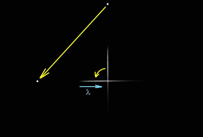
The wavelength calibration reference spectrum (called "neon" in the dialog box) is  here just one of the spectra of the sequence to be processed (we chose the first of the series  @ delta cas-1).  It may seem strange to calibrate a spectrum with itself! The explanation is that we will use the zero order image as a standard line to determine the wavelength of all other points of the spectrum.  This zero order image is present in all 2D spectra to be processed.

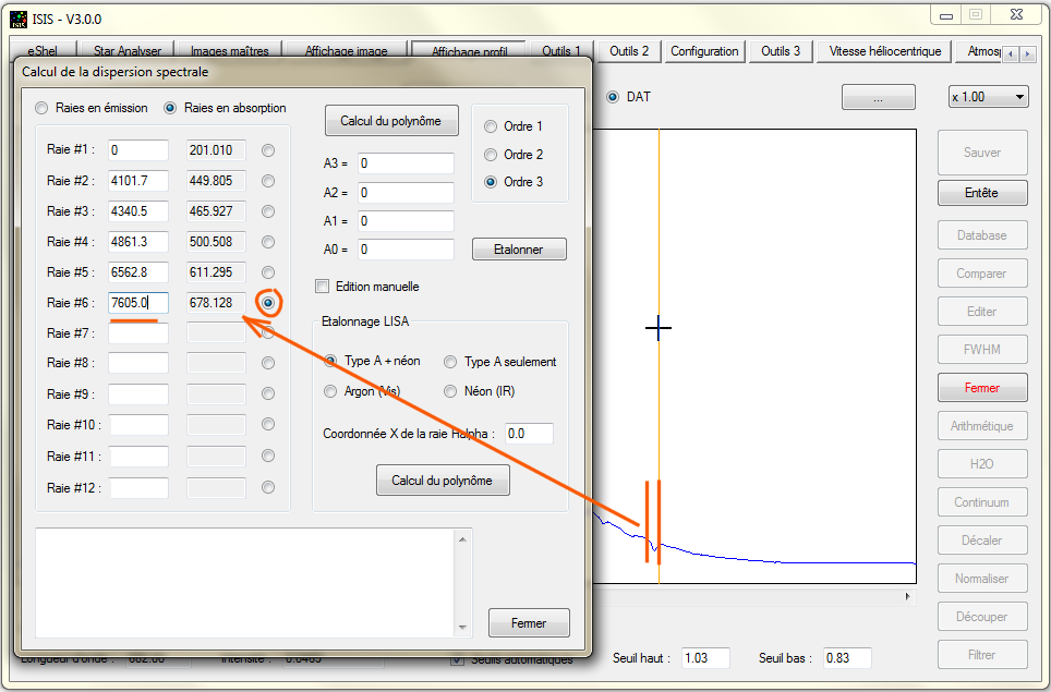
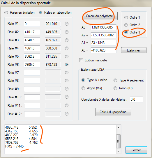
It should be noted how "spectral calibration mode" was filled in  We use the spectral dispersion law found in step 6. The option "polynomial preset"  is selected.

Note: ISIS will look for the coefficients in the dialog "Dispersion", accessible via the tab "View Profile". For example, if you manually edit these coefficients, it is these changed values ​​that are used by ISIS during the spectral calibration.

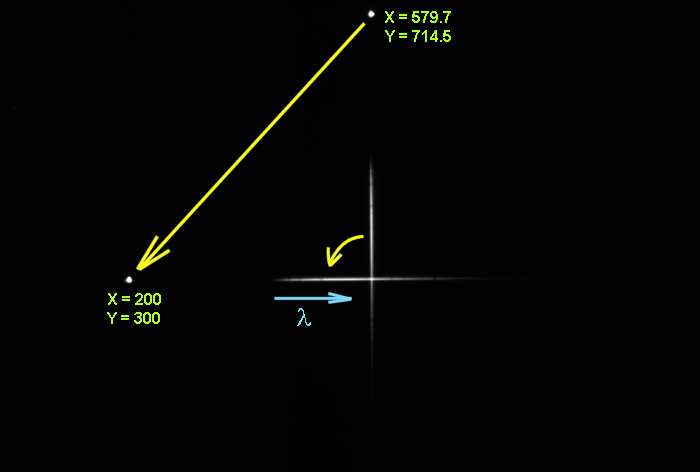
Also in the definition of spectral calibration mode, we must provide the horizontal coordinate (X) of a spectral line of known wavelength.  We use the pseudo zero-order line, which is at wavelength  0 angstroms, which by definition is at the coordinate X = 200.

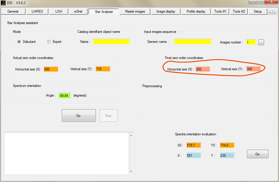
Elsewhere in the General tab, be sure to define the vertical coordinate of the spectrum (Y).  Here Y = 300, (normally this field is already pre-filled).

Give the pixel size of the sensor. Here a KAF-3200 CCD which have a native pixel size of 6.8 microns, but here used in 2x2 binning mode, so the value is 13.6 microns as  indicated.

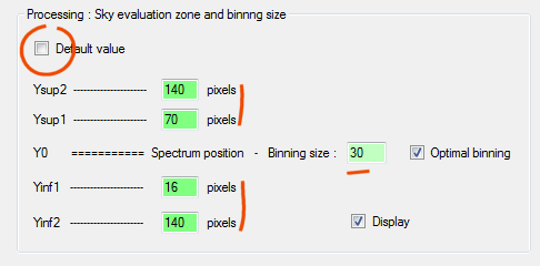
X1 and X2 define the limits of a zone (in pixels) within which the intensity of the spectrum is relatively strong.

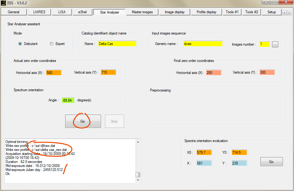
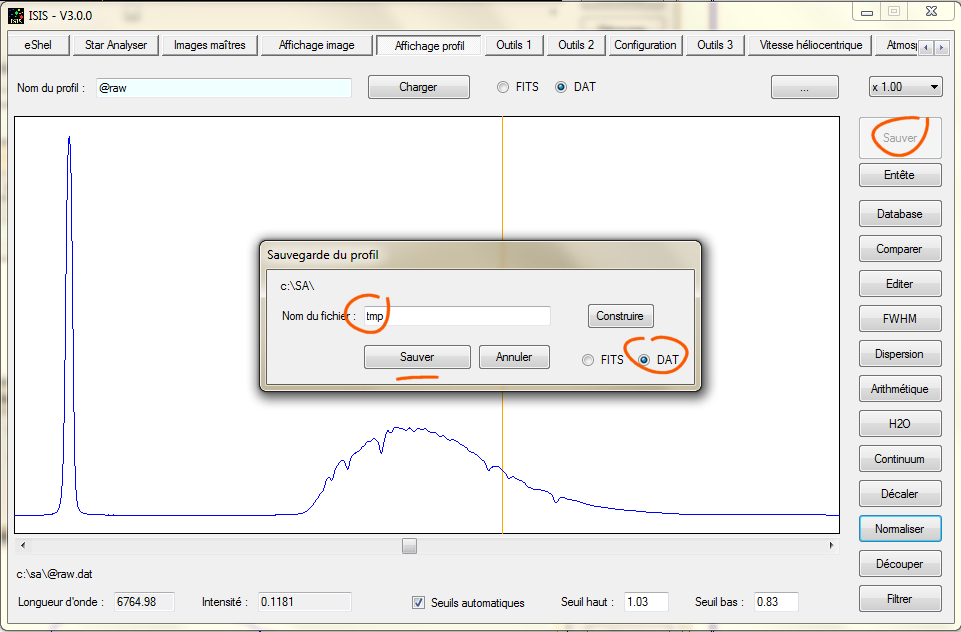
It remains only to click on "Go" and you end up with a spectrum identical to that produced by the assistant " Star Analyser", but this time directly calibrated in  wavelength.

All your spectra of the night can be treated in the same way  just using the same law of dispersion.

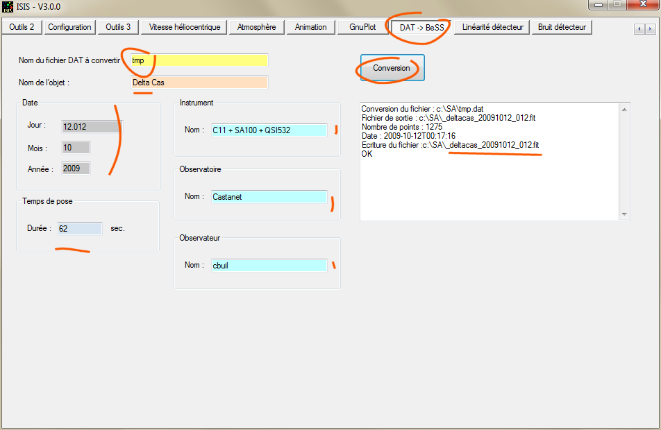
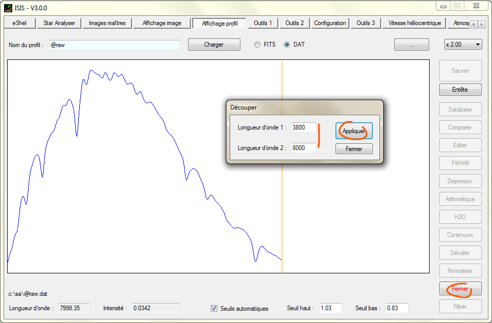
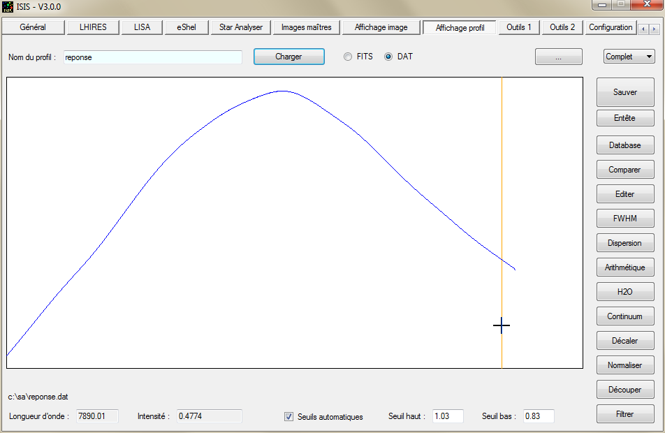
For information, the figure29 shows the shape of the instrument response found by dividing our spectrum (cropped to its useful part) by the expected spectrum of a star type A5V ( Pickles database, accessible via the ISIS tab "View Profile").

You can then resume processing generally, but this time taking into account the instrumental response, as shown in Figure 30. The spectral profile obtained is then the true profile of the star.

Figure 27.  One of the 2D images from the pretreated sequence. It shows the approximate location of the zero order (within a few pixels).



Figure 28. viewing the pretreated 2D spectra from the "General" tab.

Figure 29. The relative spectral response of the instrument.
 


Figure 30. Treating the spectra to take account of the instrument response.