
Quick Start (part two)
In the set of Valerie's images, you can find the file DARK10_5.FIT. It is the thermal map of your CCD dectector.
This is the average of several exposures performed in total darkness with an exposure time of 10 seconds and detector temperature of -5 °C (same condition during science images acquisition). ISIS has tools to calculate effectively this type of master image, but the subject is out of this quick introduction (see "Master images" tab).
Visualize the "dark" image from "View Image" (below screen copy). You must adjust viewing thresholds below 1000 ADU value because the low intensity of the image. Normal, since it is acquired in darkness condition :
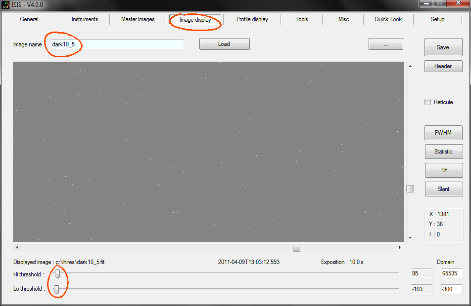
Tip: In some circumstance, the threshold sliders adjustment for modify contrast and brightness may be too insensitive. You can easely modify cursors excursion for cover these situations. The default values are in the range 0 to 65000 ADU (Analog Digital Unit). For the example, the setting is between 0 and 1000. It is also quite possible to indicate a negative value for a threshold, -500 for example, which offers the ability to better perceive very faint details of the image, which a level intensity close to zero. Be careful, think back to a large excursion if you view bright pictures, otherwise you always display white.
Now the offset image :
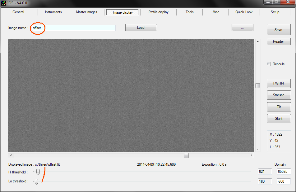
An important operation of processing pipeline consist to eliminate offset and thermal signal. The operation is simple: we subtract offset image and dark (thermal) image from each raw star. The quality of the extracted spectrum will be even better. From "Quick Look" tab, enter the offset and dark (thermal) image name, then click on Go button.
Processing is always fast. Note that in the output window, ISIS indicates that subtraction of dark frame is now taken into account.
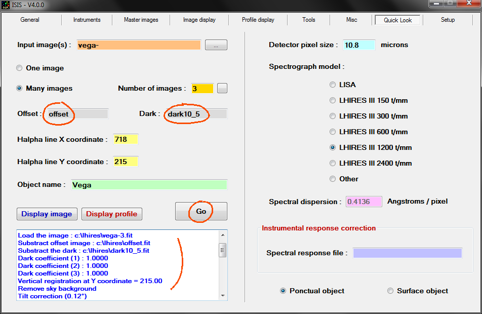
Tip: The file is named dark10_5 because it is an exposure of 10 seconds in darkness with a CCD temperature of -5°C.
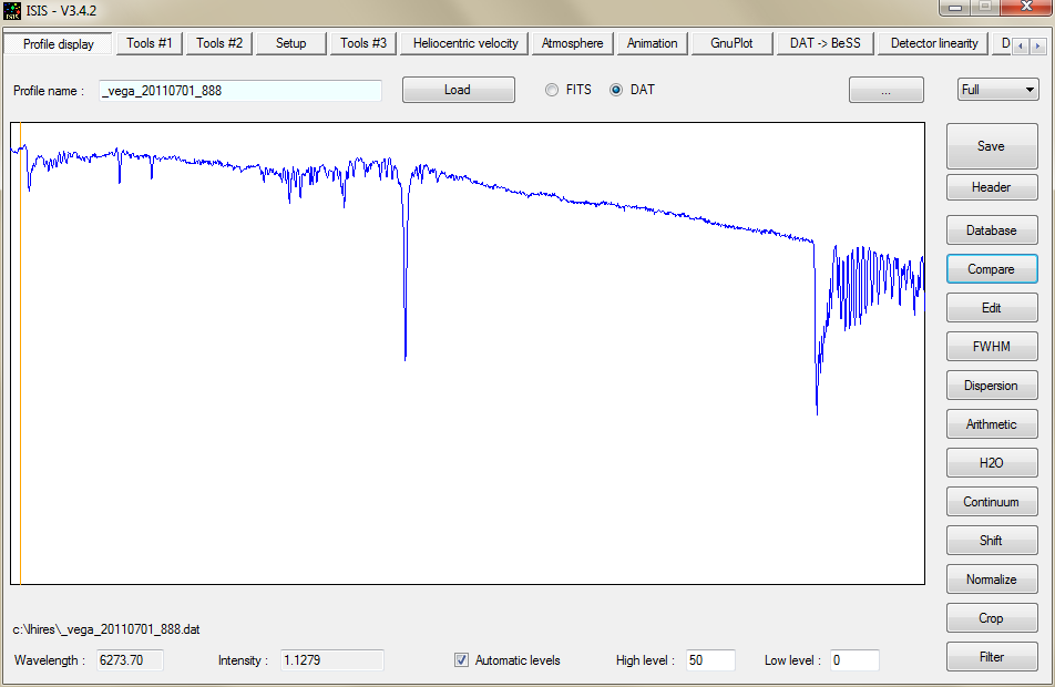
If you display the resulting spectral profile (View spectrum button), positive effect of dark frame substraction is not very evident. But he become clear when you take spectra of vey faint objects with long exposure.
The actual Vega spectral profile not accurately represent the true flux distribution as a function of wavelength that reaches us from the star. This is unfortunate. The problem is the telescope, the spectrograph, and even the atmosphere. These elements act as spectral filters that attenuate the spectrum differently in function of the wavelength. Our job now is to find the exact spectrum, as it could be observed from the vacuum of space and with a perfect instrument. ISIS has an integrated spectra library which provides expected profiles for various spectral types, including the type A0V, the spectral type of Vega.
Note : the procedure for install ISIS specral data base is described here.
Click Database button from the list tools at the right edge of the "Profile display" tab :
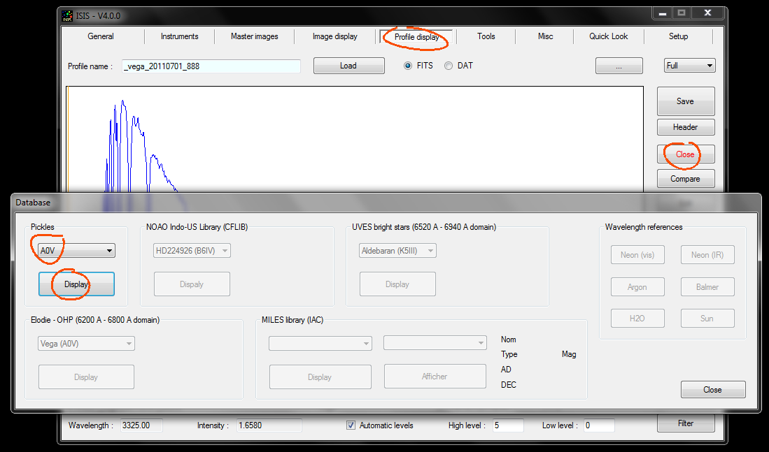
Choose from the dropdown list the A0V type, then click Display button.
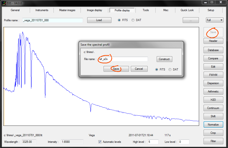
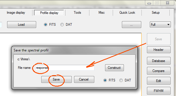
We will save this profile in the working directory as an intermediate file. We choose a file name easy to remember, example: REF_A0V (i.e. reference spectrum of a theoretical A0V type star).
Click on the Save button of right tools bar, as shown in the folowing screen copy. In the dialog box, enter the file name, select the DAT format, then click Save button of dialog box. A new file appeared in the working directory: ref_a0v.dat.
Note: The spectral profile is saved by the following procedure is the actual current spectrum displayed on the screen.
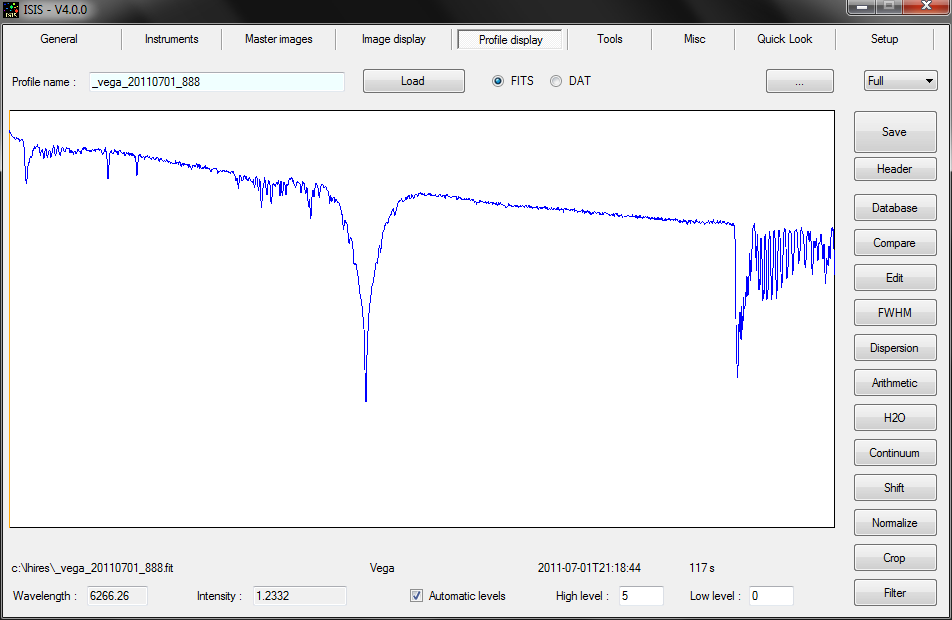
The contents of the file _vega_20110701_888 appears on the screen. We will now compare the observed profile and the theoretical A0V profile.
To do this click the Compare button of the toolbar. The dialog box that opens ask you to compare two spectra, the current spectrum (observed) and the refence A0V spectrum.
Click the Compare button. The compared spectrum appears in superposition of observed spectrum. They are distinguished by the colors :
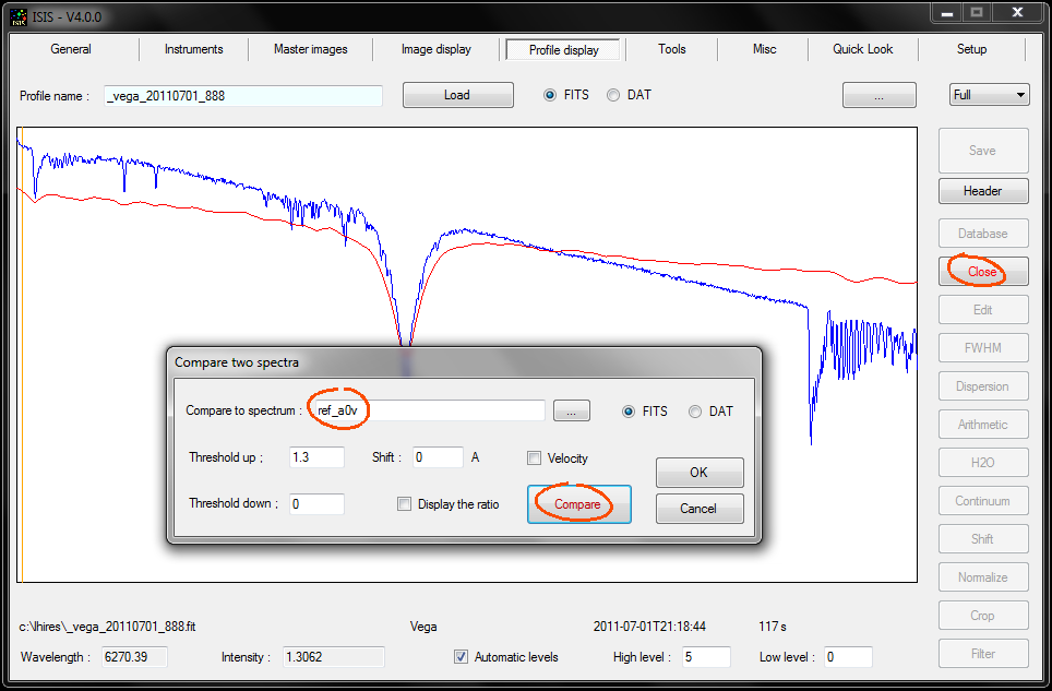
You can adjust the visualization contrast by changing the threshold values. You must click Compare to take your change into account.
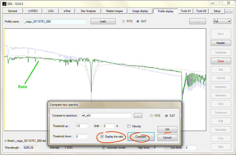
The spectral resolution of Valerie spectrum is typically 5 times of the Pickles spectrum. This is a problem, but we going to do with (ISIS integrated data base offers more resolved spectra, but their use is beyond the scope of this tutorial).
The ratio shows residual telluric lines (H2O, O2) present in our spectrum of Vega, but not in the Pickles model. The Halpha line remains visible in the ratio, because the spectral resolutions are not identical in the two compared spectra. We will treat this problem below. The general form of the computed ratio is the instrumental response.
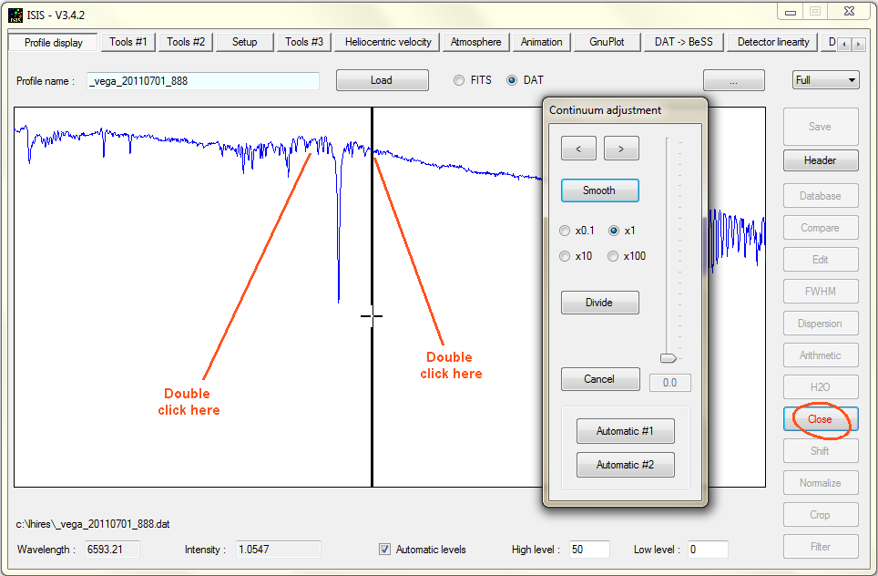
We will conserve this ratio. To do this, click on OK button of dialog box (or Close button of "Profile display" tab toolbar).
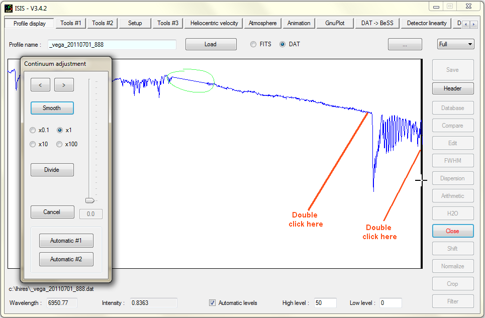
A new dialog box is open. Double click (left mouse button) then the pointer is a little at the left of the Halpha line residue. The only apparent effect for the moment is the appearance of a wide black vertical bar that moves with the mouse. Make a new double click, this time at the right side of residual Halpha line.
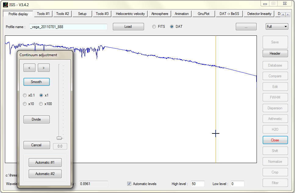
It remains rapid fluctuations in the profile ("high frequency" details) that are associated with low intensity telluric lines (produced by water vapor in our atmosphere) and noise in the observed spectrum. While it is possible to delete faint telluric lines manually, we adopt a different way: ISIS can smooth the spectrum for a nearly equivalent result. Simply click on the Automatic # 1 button of the dialog "Find the continuum." The result is displayed in blue :
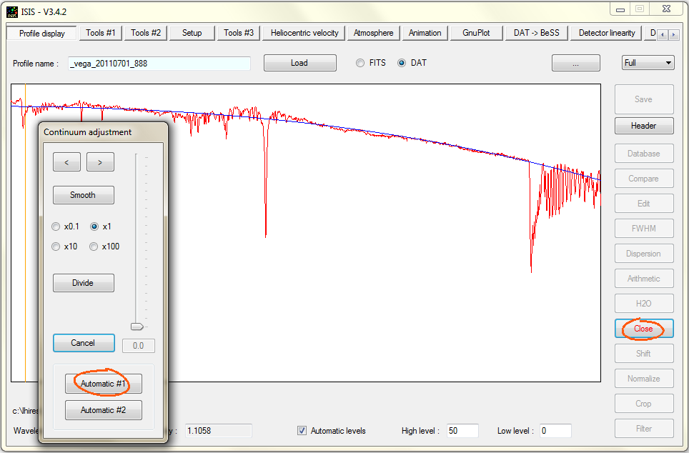
Tip: The Automatic #2 does the same thing, but the smoothed profile follows more closely the original profile. You judge the best option for fit the best continuum. This choice is often somewhat subjective.
Exit the dialog box by clicking Close button on vertical tools bar of "Profile display" tab.
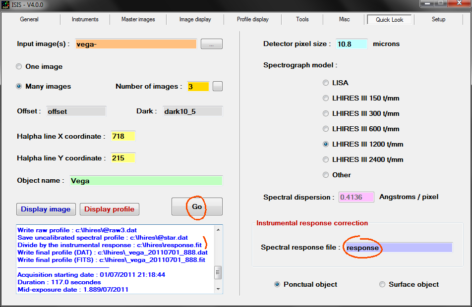
Tip: The instrumental response is a feature associated to your own instrument, a constant for it. You can use it to process another star.
Give the name of your instrumental response, then Go :
The
quality of the produced result at this stage is good. But for excellence (high calibration
precision, optimization of signal
to noise
ratio, ...),
for generate a scientifically exploitable
spectrum, please
read ISIS
full documentation... and
experiment.