| Nothing like a good pratical
application to learn a new
tool! It is recommended
do this exercise yourself, you grow much faster.
You can download the set of spectrum images
(vega
star + calibrating imamgs) by clicking
here (5 Mb). Unzip and copy the contents in
your working
directory (here
C: \ LHIRES
- an example only).
Note: Concerning the working
folder, of course you have the
freedom to make a
whole other choice. For example, I usually
create a
directory per
night, with for
the name, the date of night observation.
We calculate the spectral profile of the brilliant star
Vega, observed with a telescope
C9.25 and a LHIRES III spectrograph. The diffraction grating is the 1200 lines/mm
model.
The CCD
camera
is a QSI583 whose
pixels
are 5.4 microns aside. The camera
is operated in 2x2
binning mode
at the time of observation
(on chip grouping native
pixels pairs), so that
the effective pixel
size
is 2 x 5, 4 microns
= 10.8 microns. The
observation was made
by Valerie
Desnoux from
the center of Paris (Saint-Charles
observatory)!
For the
moment we will porcess only
first
spectrum of the
Vega sequence.
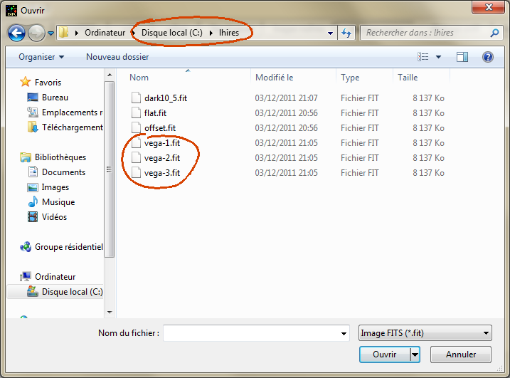
Valérie has
captured three
successives spectra of Vega.
The exposure time for each frame is 10
seconds. You
can note also presence of other files,
usefull for a complete pre-processing of spectra. One corresponds to
CCD offset signal (image obtained in a very
short exposure
time in the
dark), another is the
dark signal associated with an exposure of 10 seconds and
for -5°C CCD temperature (file dark10_5.fit) and
finally response of
all pixels to
a uniform field placed in front of the telescope (image flat.fit). |
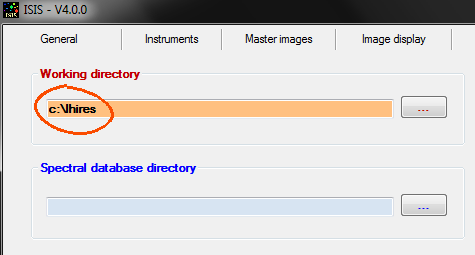
We
indicate now to ISIS
the location of images
to be processed.
The information provided in ISIS can
be written
in lowercase
or uppercase. It is indifferent.
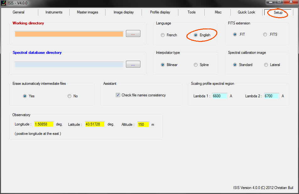
Select the "Setup" tab,
then fill in the Working Directory
field as
show in the
screenshot to the
right
Tip: You can press the small
button at the right of the corresponding field
("...") button to select
interactively working directory.
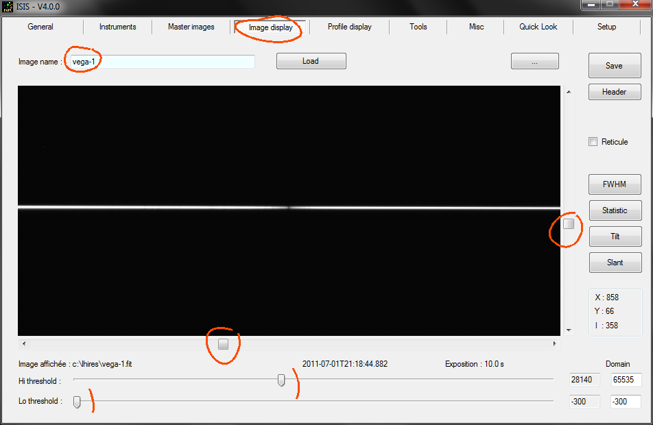
Consider the appearance of the image
vega-1.fit. It
is such that at the time of acquisition. It is a raw image. Go to
the "Image
display" tab. It
is a strategic
location in
ISIS: To
view the contents of
any file image, you must go here.
Enter the name of the image to view in
the field Image
name
at the top of the
window. Note that it is not
necessary to indicate the image
path. ISIS knows
that your images are located in the directory
C: \ LHIRES. Similarly, you do not have to indicate
the extension file type (. fit).
Tip: It may happen that the extension of
FITS files is ".fits". Go to the
"Setup" tab and choose the
correct extension for you file.
To
confirm your choice
for image
file to display, you can press <Enter>
keyboard or
click the Load
button.
You can also use the classic
file selection dialog box,
usual
in Windows,
by clicking the button marked "
... ".
The
spectrum itself does
not appear necessarily clear in the visualization area. You must adjust the vertical horizontal displacement
sliders and
the visualization
threshold sliders
(later act on the contrast
and intensity displayed).
The spectrum is a narrow and
approximately horizontal. Only the Halpha
hydrogen line
becomes clear
toward the center, in absorption. This is the spectral region
chosen by
Valerie, around the famous red hydrogen
line.
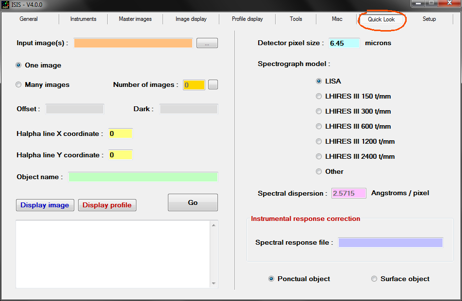
After this
first contact with vega-1
image, open the tab from which we
will run majority
of
operations in this tutorial. This is the tab "Quick
Look
".
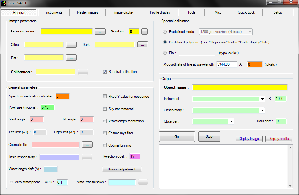
Our job now will be to fill
some
fields needed to
extract the spectral
profile...
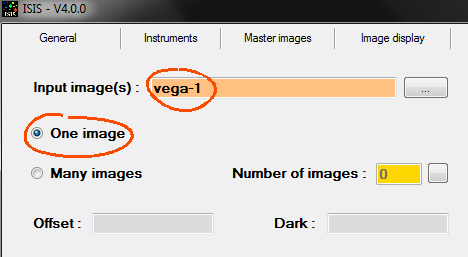
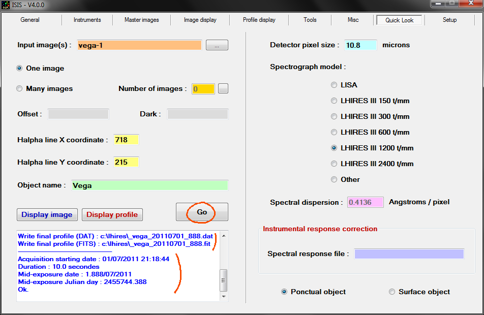
In
the field Input
image(s), enter the
name of the image to process: VEGA-1
(in lower
or major case).
Do
not indicate directory or extension
for the file image name. ISIS will build
for you
the full name "c:\lhires\ vega-1.fit".
We process for
the moment a single image. Indicate
this by selecting
One
image option. See
the
screenshot below :
Do not worry
about the field Offset
and
Dark.
Leave blank for time.
We must now provide the horizontal (X axis) and vertical
(Y axis) of the hydrogen
Halpha line in
pixels
from the input
2D raw image.
Returning to view this image. To do this you can select
the tab "View image",
or faster, click on Display
image button
from "Quick Look" tab:

If
you move the mouse
pointer in the image, you will see that ISIS
returns
the current
X and Y
coordinates (the cursor takes the form of a thin cross) and
the intensity of the image there. The origin of the coordinate system is
located in the lower left corner of image (and starts with the coordinates
1,1).
Tip: The arrow keys
of keyboard can move the mouse pointer very precisely.
Your only
job is to make a
Double click with
the left button of
the mouse
by positionning the cursor
cross on the Halpha line.
Try to
this with
some precision, one
pixel error
max if possible, especially along the X coordinate
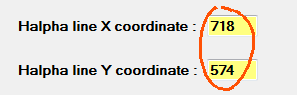
(horizontal axis). In our example, the coordinates of the
Halpha line in the image are X
= 718 and Y
= 574 : 574.
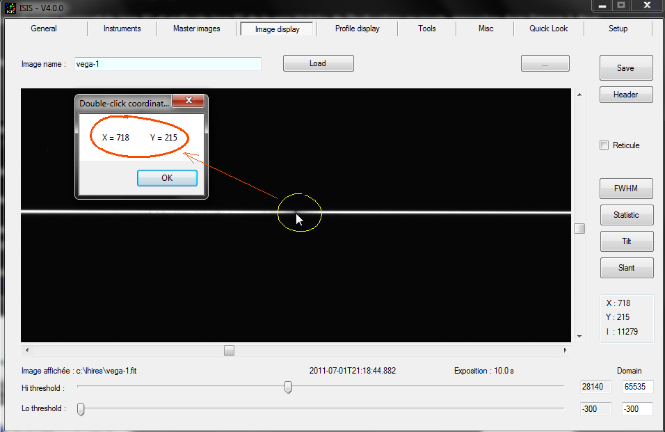
Open
the "Quick
Look"
tab. ISIS has completed
automatically the fields X and
Y after the
double clicking (without
the double
click, you
have to write these coordinates by hand) :
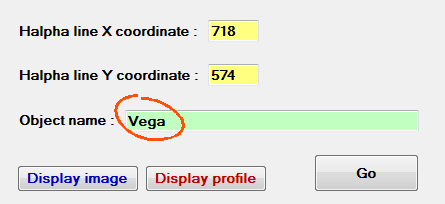
We
must decide the name
for the spectral profile that will be generated by ISIS. Ideally,
the file name should reflect
the object name. Here please choose enough
logically:
Vega.
Note that this time we
made the distingo
between
upper and lower
case. The name of the object in the
FITS header file produced is exactly the name you enter now.
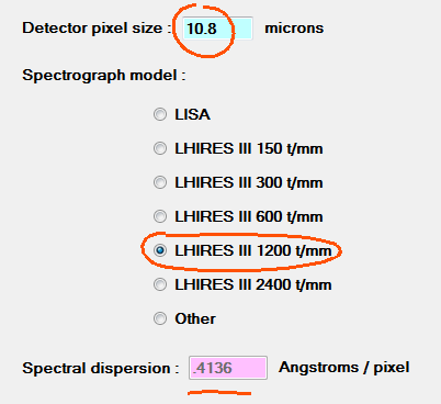
Indicate the pixel
size.
Here the value is 10.8
microns
(remember, we are
in 2x2 binning
mode).
Then
select the name
of spectrograph used.
ISIS calculates the spectral dispersion
expected in the spectrum in Ansgtroms per pixel. In the example, ISIS
returns an
average
dispersion of
0.4136 A / pixel.
Tip: If your spectrograph
model do not appears in the list, you
can enter manually the mean
value of the dispersion
by
selecting Other
option.
You
can now start
processing by clicking the Go button. The operation duration
is only one or two seconds.
ISIS returns to the status
window some
infos about the processing. The spectral profile is saved in the
working directory both as a FITS file (binary
form) and as both a
DAT file
(ASCII
form). These two files
are distinguished by
their extension
(. FIT
and . DAT
respectively).
The result files are always built
in the same way by ISIS:
_ "OBJECT NAME" _AAAAMMJJ_FFF.FIT (or . DAT)
The name of the concatenation
of object name and
date, indicating the moment of
beginning of the observation.
The output window gives much more
information, whose meaning will be decription throughout the
ISIS documentation.
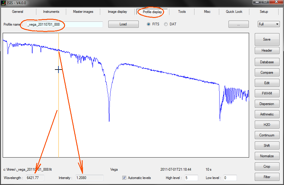
It is probable that you would like to see result. Click Display
profile button....

The tab "View
profile" opens
automatically, with the spectral profile already drawn - as in the screenshot below.
The spectrum is wavelength
calibrated.
Proof, if
you move the mouse pointer, the wavelength in Ansgtroms
unit is
returned in
real time. If you position the mouse pointer
at the level of the Halpha line, you must
find a wavelength of about 6563 A, which is effectively the
correct value.
Familiarize yourself with some functions
present in this tab. For example, notice that the
fields Profile
name
is already pre-filled.
ISIS actualize
the field contain during the processing
stage. You can load into memory and display any valid giving spectrum
by given its name
- than click Load
button (or <Return> from
keyboard). It is your responsibility to select
the good spectral file formal : DAT or FITS. Of
course, by
clicking on the
button "
...
"
you display a dialog that facilitates the search of the file
in the disk. The identification of the files is more visual.
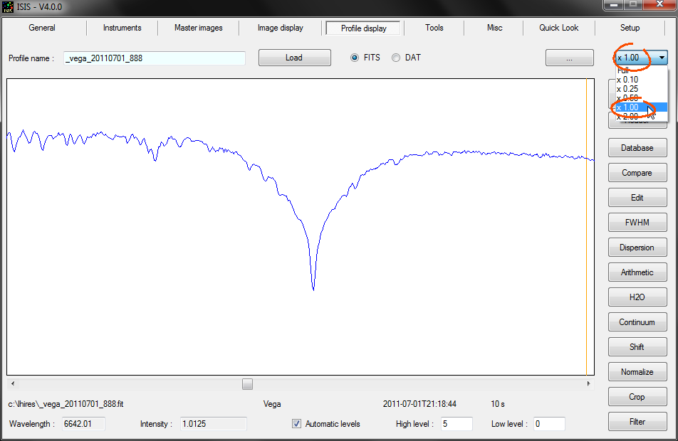
To
enlarge the
profile (zoom
effect)
scroll down the list at the
top right of the tab "View Profile" and
select
a magnification factor.
The spectral profile can
be tuncated at the right and
left of the visualization window
according to the zoom
coefficient chosen. Use then the bottom scroll bar
for explore the various part of the spectrum
:
Return to the "Quick Look" tab
and
click this button:
The 2D image which was extracted the
spectrum profile
is
now visible.
This displayed image is not the original image VEGA-1.FIT. It is a processed version of
the
latter. Besides, look
at the file
name that appears at the top of the window :
_Vega (. fit)
This name
is constructed by preceding the
object name with the character "_". ISIS shall always in
the same maners. The
file is present in the actual working directory :
ISIS rectify
geometry of the raw file (the spectrum
trace is now perfectly horizontal), remove the sky background (see full documentation for more details), .... Also ISIS extract the spectral profile of this 2D
image using a
special algorithm that minimizes the noise in the profile.
If you
work a sequence of
images of
same star, not just one, the image
_OBJET.FIT is the sum (processed)
of these individual input
2D images. Precisely, we process now
simultaneously the 3 Vega images captured
by Valerie
The
operation is of great
interest since equivalent exposure
time is multiplied by 3.
We can
therefore expect
a better spectral profile. We
will check
...
Open the tab "Quick Look". Select
Many images
option and provide the number of images (here 3).
Tip:
The number of images
available
can be
calculated automatically by ISIS if you click the little button at
the right of
field Number of
images.
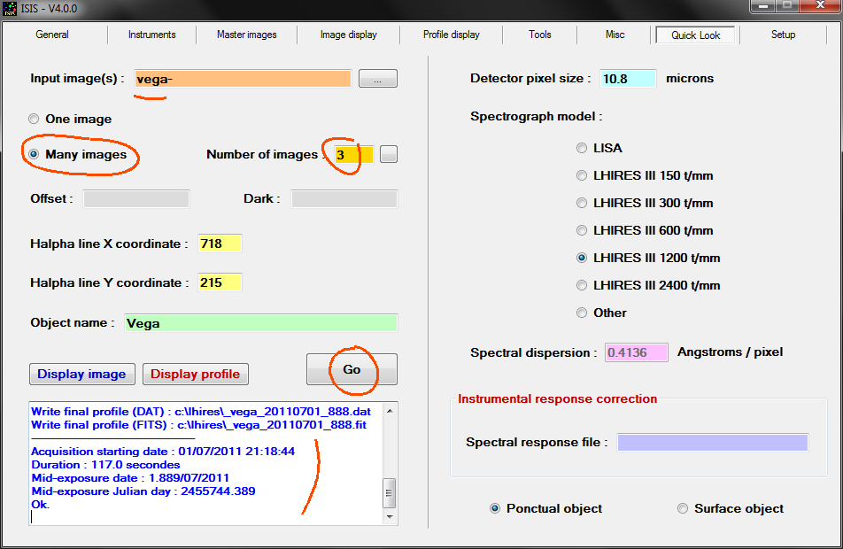
Look carefully the image input name : VEGA-
The
index number is now removed because ISIS add automatically index "1", "2"
and "3" during
processing phase. This mean
ISIS will load and process images:
VEGA-1
VEGA-2
VEGA-3
The form "VEGA-" is called a
generic name
in ISIS
language.
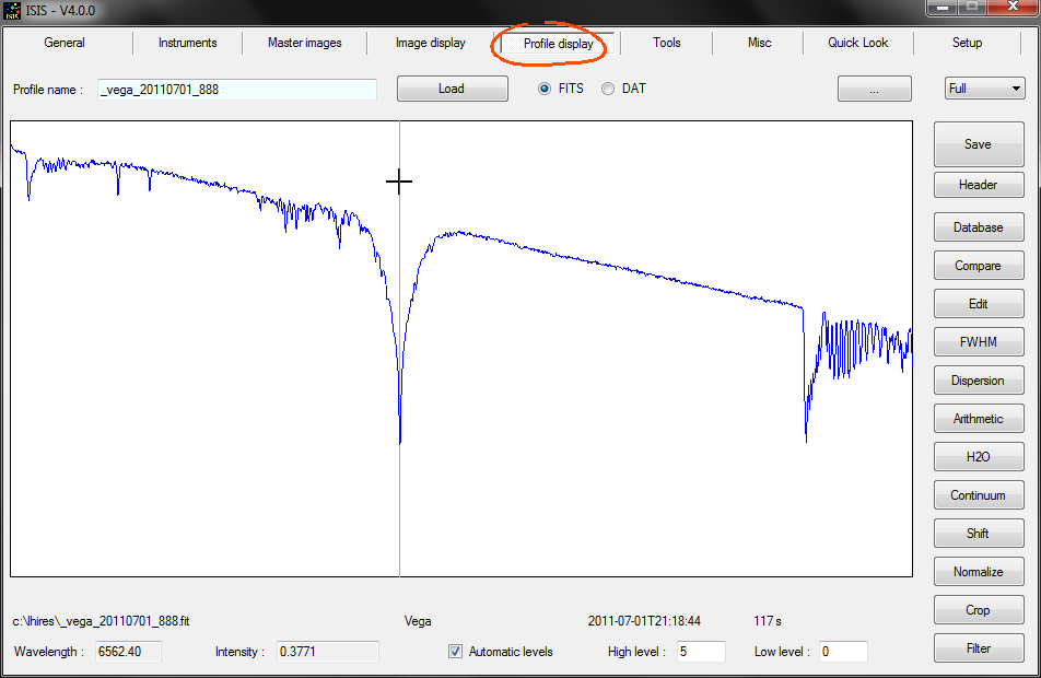
Click Go, then
view the
profile by pressing the
button:
Since we merged information
three images distincts
spectral images, the noise
(random fluctuation) in the
profile is lower.
Remember, the exposure time is now 30 seconds and not 10 seconds.
We
end here this
quick
start with ISIS.
You have just
discovered important
functions, and indeed you have gone through the largest path in learning of
this software.
But...
have you
noticed that there are
some fields that
we have not yet filled in the "Quick Start"
tab? If you want to find out what
they contain, then go here to spend a little time to discover
more about ISIS...
|