Spectroheliography
Part 1: Processing with ISIS software
Part 2: Observation with Alpy 600 spectrograph
by Christian Buil

This page describes how to use ISIS software (version 5.8 and upper) to process data acquired in spectroheliographic mode. It is recalled that this technique consists in acquiring successive spectra and at a regular rhythm whereas the image of the solar disk is continuously scanned on the spectrograph entrance slit (see the image below). The movement of the sun is obtained either by stopping the motor drive of the equatorial mount or by changing the tracking speed. For further details on this technique click here or here (Lhires II observations).

The electronic camera to be used is a model capable of producing a regular video stream at a relatively high rate. In this case, I used an ASI1600MM (ZWO) model equipped with a Panasonic mn34230pl CMOS sensor. A camera such as the ASI178MM, with a more modest size detector, would also be perfectly appropriate (and even more pleasant to use because the acquisition computer is significantly less demanding). For spectroheliographic observations, the acquired image zone is circumscribed around the spectral line of interest (the Halpha line), which frees disc space and fluidifies the acquisition.
The capture software (FireCapture) produces a SER video file, which preserves the 12 bits dynamics offered by the ASI1600MM camera. This file can be read by ISIS software to extract the individual frames, we will see how later.
I obtained the data from this demonstration during an observation made on November 26, 2016 (Castanet-Tolosan). The conditions were difficult: sun near the horizon, very strong turbulence and imminent arrival of clouds. The telescope used is a C8 (Celestron) equipped in front with a Baader Astrosolar attenuator filter (photographic version). The spectrograph is a Lhires III model mounted with a of 2400 lines / mm grating and a slit of 18 microns wide. A 7-nm Halpha filter (2 inch diameter) is placed at the front of the camera for reduce stray light effect generated by the spectrograph. The photographs below show this equipment.


The processed file is of type SER (in this format, the successive frames are coded in a simple way on 16 bits). The tools for extracting data from this type of file can be found in the "Tools / Video" tab. One of these tools returns the size of the frames and the number of frames in a SER file. In the example to the left, it is noted that the file "Sun_101312.ser" contains 1125 frames.
It is possible to extract all the frames of a SER file into a sequence of individual FITS images, as shown in the example on the right. Note that the tool in question makes it possible, if requested, to perform a cropping (delimited by the coordinates (x1, y1) - (x2, y2)). In the example, a sequence i-1, i-2, i-3, ..., i-1125.fit is produced in the working directory. It is also possible to decode only a portion of a SER file (one then gives the rank of start and end frames). The value of the step corresponds to the sampling interval of the interval thus defined. ISIS average the frames in this interval, which is a way to reduce any noise.

Note: You can choose to extract only one frame of rank N in a SER file by doing for example:

The shape of the lines is very strongly curved in the spectra resulting from the LHIRES III spectrograph because of the out-of-plane configuration adopted in this instrument. This is the "smile" effect. On the left, the image of one of the frames among the 1125. The curvature of the lines is clearly visible. It must be rectified.


A tool is specially available in ISIS to correct the smile effect for all images in a sequence. The parameters of the distortion are found by successive tests (the SMILE command exists online to help you). Here the parameters are a curvature radius of 19000 pixels and a coordinate of the center of the figure of smile to Y = 0 (approximately). The goal in fixing these parameters is to obtain straight lines and vertical lines, as shown in the example to the right.


After correcting the geometric distortions of the lines, we can now address the question of obtaining the composite image. The "Scan2Fits" tool is used, as illustrated above. The desired result is shown on the left, after converting the images of the scanning sequences i-1, i-2, ... into a monochromatic image, here called "t.fit" (arbitrary choice). The latter is 1125 pixels wide and is strongly distorted between the vertical and horizontal axis because of the choice of the acquisition frequency with respect to the speed of travel of the solar disk on the input slit of the spectrograph. Since it is desired to isolate the information contained in the Halpha line, this coordinate X represents the center of the line in question along the horizontal axis (here X = 492).
A more exact proportion between the axes is obtained by applying a different scale factor between them via the command line SCALE and applying this calculation to the image previously acquired.
The syntax of the SCALE command is:
> scale [input] [output] [x_factor] [y_factor] [mode]
It is here chosen to stretch the image by a factor 0.8 along the horizontal axis and by a factor 0.125 along the vertical axis. The image thus rectified geometrically, which is called "r.fit", is calculated by making:
> scale t r 1.6 0.25 2
(The last parameter sets the interpolation mode during the calculation. Mode 2 offers optimum quality for the type of operation performed). The result is shown opposite.


The same operations are extended by isolating this time a part of the spectrum without spectral line so as to obtain a continuum picture. this is called (for example): "continu.fit". It generates by using again scan2fits tool (note the new value of the X coordinate, here X = 432). This image of the solar continuum is made at the same scale as the H-alpha image.

The continuum calculated image of the solar disk.
We will exploit this continuum image to correct the transversalium (horizontal streaks related to slot width irregularities) and non-uniformity between the top and bottom of the image (internal vignetting of the spectrograph). A sun spot free zone is selected towards the disk center, here between the coordinates X = 300 and X = 400, and then the correction of the transversalium is applied to the image r.fit (Halpha image), as shown on the right. The value of the coefficient is the characteristic intensity of the image "continu.fit" between the coordinates [300-400]. The threshold defines an intensity value in the image to be processed (r.fit) below which the correction of the transversalium is not realized, which avoids producing artefacts.

On the right, the "rr.fit" image of the solar atmosphere after correction of transversalium defects.

At this stage it is possible to decide to sharpen the image better to eliminate edge effects and areas that appear to be too affected by noise. Here we will perform a windowing (cropping). The CROP command is used for this purpose, the syntax of which is:
crop [input] [output] [x1] [y1] [x2] [y2]
We do in this case:
>crop rr c 1 29 740 313
which gives the result displayed below.
It can be seen in this document that the solar disk during acquisition did not move in a direction exactly perpendicular to the long axis of the slit. This explains why the right edge of the disc "falls" in relation to the left edge. It is possible to correct this geometrical defect by practicing a distinct sliding of the lines according to the column of the image (SLANT type correction).
To lose no information in the operation, we begin by adding a little space at the top and bottom of the image "c.fit" by producing the image "cc.fit" and by using the online EXTEND command:
extend [output] [input] [dx] [dy]
Here we add a black area of 25 pixels at the top and bottom of the image by doing:
>extend c cc 0 25
Here is the result :
Finally, we use the SLANTY command, whose syntax is:
>slanty [input] [output] [x0] [alpha]
With x0, the horizontal coordinate of the rotation pivot (the center of the image is chosen here), and alpha, the angle of rotation (found by successive try). Here we are going to make x0 = 350 and alpha = 1 °, hence the command:
>slanty cc final 350 1
At the right, the result.

All you have to do is set the north up using the "Image permutation" tool on the "Image processing 1" tab. See the result on the right (note the indication of a null image number to prevent ISIS from performing an indexing).

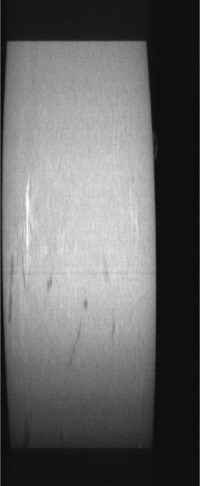
Here is our final image of a portion of the solar disk. If necessary, other scans can be made to constitute a global image of the solar disk by a mosaic technique.
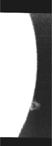
Image of the solar limb displayed in high contrast to better demonstrate the presence of a protuberance.

Part 2: observation with ALPY600 spectrograph
The Alpy 600 spectrograph (Sheyliak Instruments) is a very compact and simple to use instrument, specially designed for the study spectra of faint objects of the sky with a low spectral resolution. It is therefore not at all an instrument suitable for observing the solar chromosphere. However, it is popular, widely disseminated and of relatively modest cost. For these reasons, it was very tempting to see what such non-standard equipment in the world of SHG (spectroheliographs) was capable of in the subject that interests us here. Given the spectral dispersion and the pixel size of the ASI1600MM camera used, the spectrum sampling is about 2.1 Angstroms per pixel. It can therefore be considered that the spectral passband is of the order of 2 A, which is notoriously greater than the 0.8 A generally accepted as necessary to start taking correct images of the chromosphere in the light of Halpha line. We will still try, and also target the H and K lines of Calcium II, notoriously less demanding in terms of thinness of bandwidth.

Vue du spectrographe Alpy 600 exploité en mode spectrohéliographe, fixé à l’arrière d’un télescope Celestron 8 lors de l’observation décrite ici, effectuée le 30 novembre 2016.
View of the Alpy 600 spectrograph operated in spectroheliograph mode, attached to the back of a Celestron 8 telescope during the observation described here, performed on December 1, 2016.

Detail of the setup. Note the simplicity and compactness for a SHG. The Alpy 600 spectrograph is equipped with its reflective slit guide module. The pointing / guiding camera is an ATIK314L with an additional optical density at the front. The input slit of the spectrograph is 14 microns wide, the narrowest currently available on this model.


Aspect of the solar spectrum in 2 dimensions realized with the Alpy 600 spectrograph and an ASI1600MM camera. The display is offered in two contrasts which favor either the blue part or the red part. The BAADER Astrosolar filter is far from being spectrally neutral, being substantially more transparent in the blue part, with a particularly sharp transmission peak around 475 nm. The spectrograph is here equipped with a slit of 13 microns wide illuminated by the f/10 telescope beam. The mean spectral dispersion is 2.1 A / pixel of the camera ATIK1600MM (used in binning 1x1). Note the slight « smile » effect on the shape of the lines.

Solar spectrum commented to allow you to identify the spectral lines. Note the Ca II lines (H & K) in the blue and the red line of hydrogen (Halpha), classically exploited to produce images of the solar atmosphere.


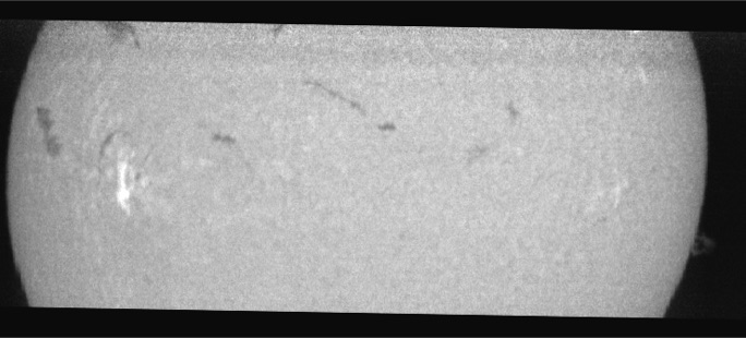
First result obtained in the blue continuum (top left) and in K line of Ca II (top right). These images are constructed by grouping 3 successive "scans" of the solar surface, assembled by image processing. On the left, a detail of the spot group in the light of the K line. During this observation, atmospheric turbulence was particularly strong. This first test clearly shows that it is possible to carry out a detailed and rich spectroheliogram in the H and K lines with a simple Alpy 600 spectrograph!
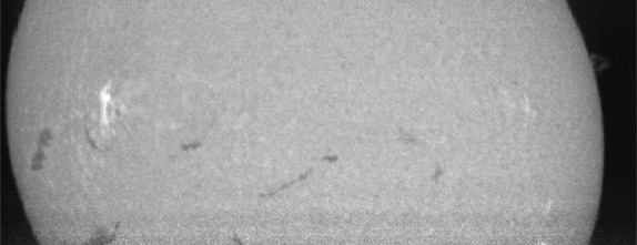
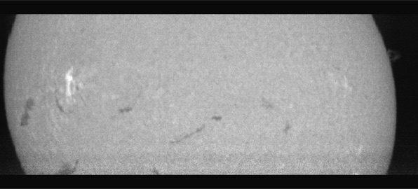
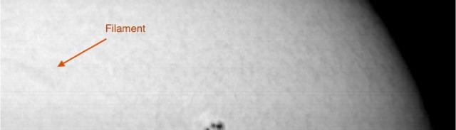
The exercise is less well engaged for the hydrogen line because of the bandwidth too wide (2 A). The observation was nevertheless tried. In the end, it is still possible to detect the faculae plage ranges on the disk (and thus probably erruptions), and one can even guess the presence of a filament in the document Alpy 600 presented in the upper part. This is not such a bad result given the type of instrument used.
For comparison, at right Halpha picture of the Sun performed at the Pic du Midi with the instrument CLIMSO almost at the same time. Copyright The Associated Observers / FIDUCIAL.

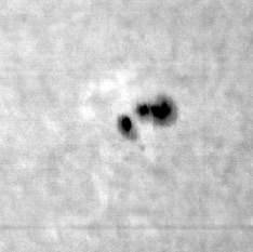
Left, detail of the spot group observed previously in Ca II H, but this time in the red line of hydrogen with a bandwidth of 2 A.
It can be concluded that any owner of Alpy 600 can try, at least on an experimental basis, to observe the solar surface and to obtain some information without having to modify his equipment and enjoy it. This multiplies the scope of this small spectrograph. It is anticipated that the availability of a narrower entrance slit (9 microns) and the use of an ASI178MM camera (for example) at smaller pixels should further improve the results presented here.
