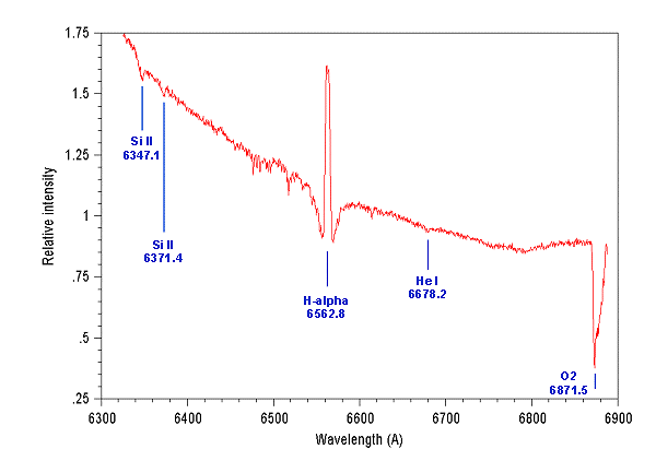
At this step, the intensities scale represents the sum of the pixel values calculated after the binning operation which has transformed the 2-D spectrum into a 1-D profile. In general the values are large and are greatly dependent of the exposure time. In order to handle reasonable values and more important to make possible comparison between spectrum acquired at different exposure time, it is strongly recommended to normalized the intensity profile. To perform the normalization process, a mean value shall be computed on a spectral zone where no lines are present. The wavelength zone is set in the preference dialog box, under the tab continuum. For the Be stars survey, this particular point is selected between the wavelengths of 6620 A and 6660 A, which is an area without any spectral lines (the intensity of the point is the average of the intensity in this spectral field). For that, it is necessary to use the Normalize command in the menu Operations. In the example spectrum, the continuum is normalized to one at the wavelength around 6640 A.
Once this radiometric calibration will be done, the intensity in the spectral profile will represent the true distribution of the signal intensity versus wavelength coming from the star.
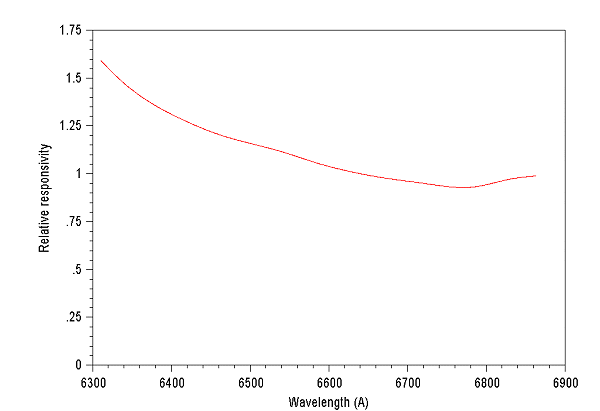
The operation thus consists in eliminating the contribution from the instrument to the intensity profile of the spectrum. To do that, the spectral profile must be divided by the spectral response of the instrument. This response is obtained by observing a star having a spectral profile which is known well and of which the spectrum is relatively free from spectral lines (we often use Vega, a convenient star taking into account its brightness, although the line Ha there is very well marked). The graph hereafter shows the spectral instrumental response calculated (standardized to 6640 A). Click here for more information about determination of instrumental responsivity.
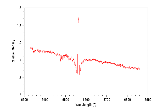
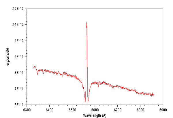
The division of the rough spectrum spectrally calibrated of HD169033 by the relative instrumental response complete the spectral radiometric calibration. It is necessary for that to use the Divise command in the menu Opération. The following figure shows the result. The slope in the continuum is now characteristic of the Planck profile of the star.
4.8. Remove the telluric lines
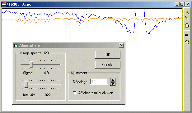
The majority of the visible lines on the left of the line Ha, but also more slightly in the sides of the latter, originate in the absorption of the light of star by the water vapor of the atmosphere. These telluric lines obstruct the analysis of the profile of the line of hydrogen and must be eliminated as much as possible. It is necessary for that to use the command H2O in the menu Radiometry which makes it possible to interactively adjust and compared to the spectrum observed, a synthetic spectrum of water (the parameters of the adjustment are the depth of the lines, the spectral resolution and a fine adjustment of the spectral shift of the real spectrum compared to the synthetic spectrum).
The figure hereafter shows the detail of the operation: in blue the spectrum of HD169033, in orange the synthetic spectrum of H2O.
Once calculated the synthetic spectrum by sticking as well as possible the profile to the observed profile, it can be divided from the spectrum of star. The following image shows the result.
For specific work it is important to translate the intensities into physical values, in erg/cm2/ s/A for example. For a given wavelength l the following formula carries out this calculation:
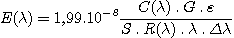
with:
E(l), monochromatic flux outside the atmosphere in erg/cm2/ s/A.
C(l), the total signal in
pixel value (ADU) by second in a spectral element (after binning
along the transverse axis) for the wavelength considered.
G,
gain of the camera in electrons per ADU.
e, fraction of the total signal of star taken into
account at the time of the binning in the direction perpendicular
to dispersion. If the quasi totality of the stellar flux is used
to build the spectral profile then e = 1.
S, the total collecting surface of the telescope
in cm2 (take
into account the possible central obstruction).
R(l), the spectral throughput of the instrument, including
the atmospheric transmission.
l, the wavelength in angströms.
Dl, dispersion in angström
per pixel.
In the example we have for the wavelength of 6563 angstroms:
C(6563) = 20,5 ADU/s (in the
continuum)
G = 2 électrons/ADU
e = 1
S = 312 cm2
R(6563) = 0,14
Dl
= 0,38 A/pixel
One finds for
HD169033 a flux outside the atmosphere of 7,49.10-12 erg/cm2/
s/A with 6563 A. It is about the typical value awaited for a star
of magnitude 5,73 of the spectral type considered.
Calculation shall be renewed for all the points of the spectrum to plot the curve of spectral distribution in physical unit.
To measure parameters of the hydrogen line, as for example the calculation of the equivalent width, it is required to normalize with a common value all the points of the continuum of star. This operation is equivalent to the first order to get to the Planck profile. In practice, some residual defects of processing can also be eliminated if needed. To go further, it can be performed an interactive smoothing like spline smoothing using the Flat command of the Radiometry menu. If needed, it is possible to eliminate the large lines before the adjustment from the continuum so that those do not skew the result. At the end of the procedure of this adjustment (the degree of smoothing of the continuum can be modified using a cursor), the spectrum is divided by the calculated continuum.
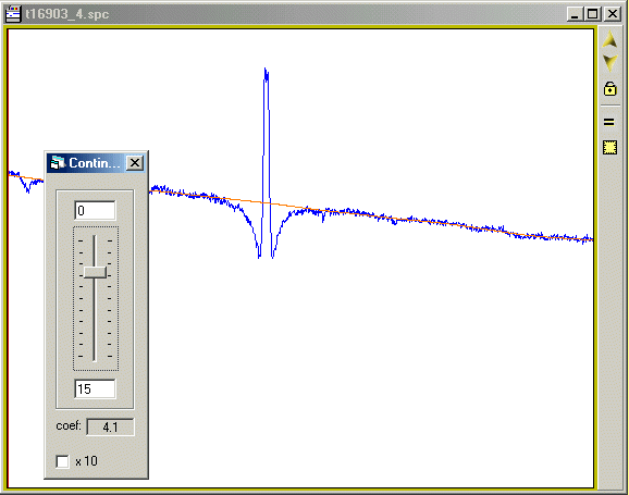
The following figure shows the spectrum after the operation of continuum removing.
At this step, it is possible to export the spectral profile in a text ASCII file in order to further exploit with other curve-processing programs or displays it in the graphics package of your choice. For that, it is necessary to use the Export command in dat in the menu File. The file created on the disc contains two columns: the wavelength in angströms and the relative intensity.
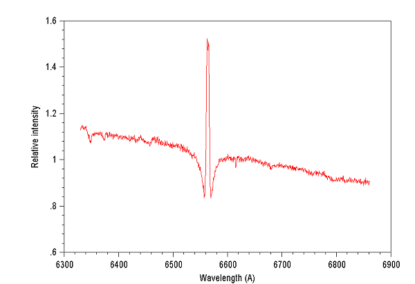
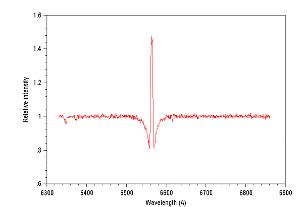
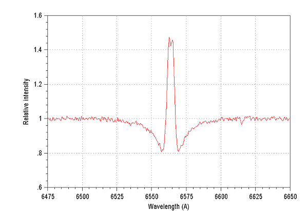
The graph hereafter shows a detail of the spectrum processed around the line Ha. It can be noted the aspect of the emission line in the middle of the photospheric line (in absorption): two narrow emission peaks are visible, probably due the Doppler effect of a cloud of gas in rotation around the star.
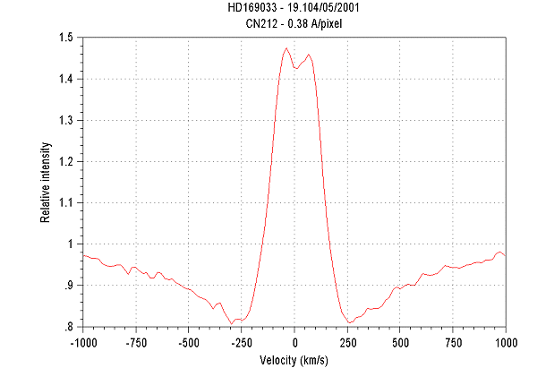
The following graph represents the spectral profile graduated in radial speed. The width of the emission line measurement gives a value of 210 km/s for the rotation speed of the gas cloud around this Be star.
Goto index page Previous page Next page