

A simple procedure for the correction of planetary limb darkening
by António J. Cidadăo
Limb darkening is a typical finding in planetary images, even at opposition, and can be considerably intense in gaseous planets like Jupiter or Saturn. It has a major role in the 3D perception we have when analyzing a planetary photograph but, interestingly, it seems to be much more illusive at the eyepiece, probably due to the "logarithmic" way our brain interprets visual information.
The limb darkening effect can be deleterious in some occasions, like for instance the production of planispheres, direct photometric measurements, and the precise determination of a planet's apparent diameter. In fact, multiple images have to be used to build up cartographic projections of planets, and to perfectly merge them together the brightness of a given feature should not change when it occupies different positions along the visible planetary disk. For this same reason, photometric measurements are usually biased by the feature's position, say at the central meridian or approaching the limb. It is not necessary for the feature to be near the limb for brightness differences starting to become noticeable, but when it is the changes can be dramatic. This marked illumination falloff at the limb often artefctually decreases the apparent diameter of a given planet in CCD images, since with "aggressive" image processing and/or incorrect image settings the outer rim of the planet may be lost in the background.
PLATE 1

Click here for a larger image (626kB)
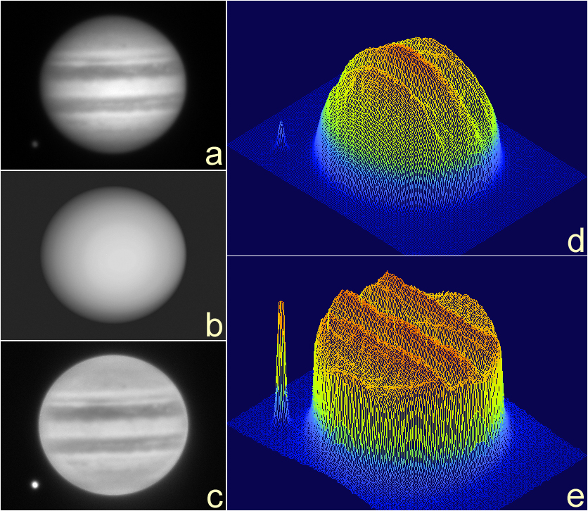
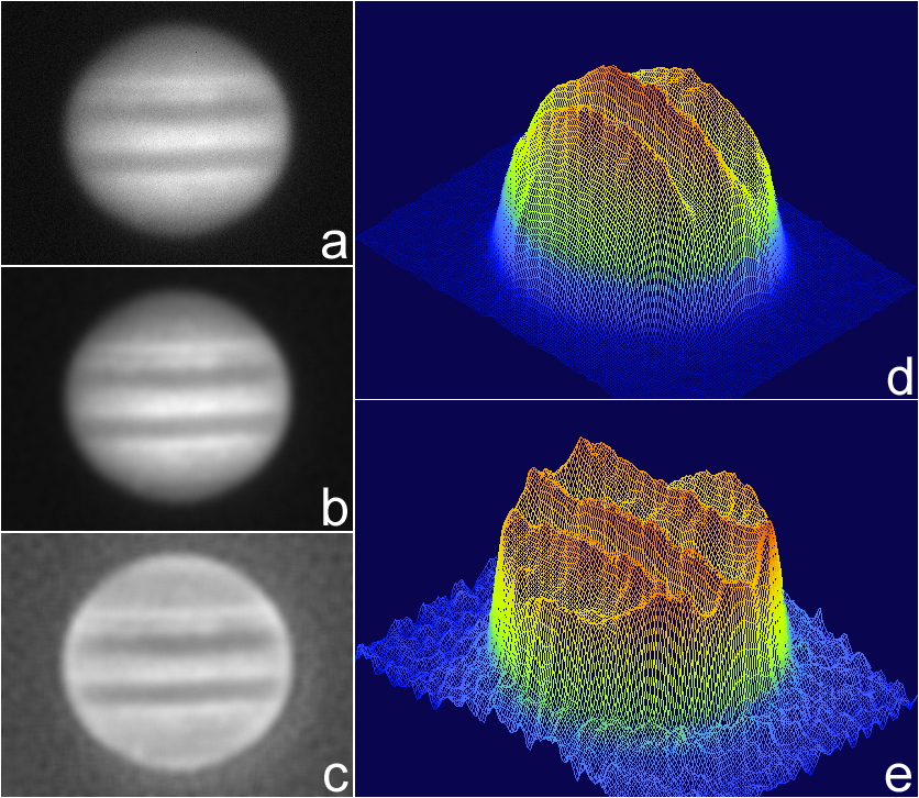
A raw image of Jupiter, obtained with a blue filter and corrected for bias, dark-current and flat-field, is shown in a). This image, obtained with good seeing and with the N up, shows evident limb darkening. The limb darkening is not uniform and, as expected from a date corresponding to post-opposition, the "f" limb at the left is less illuminated. Ganymede is also visible near the "f" limb, and started transit some time after the image was obtained. In order to correct for limb darkening, the raw image a) was divided by the custom-prepared elliptical "mask" shown in b). The resulting corrected image is shown in c). Notice the "flat" appearance of the planetary disk following the correction, how closely the image looks like a drawing and how it seems to be "larger" than the original image a). The latter observation is an illusion due to the heavy limb darkening of gaseous planets, but with "aggressive" image processing and incorrect image settings the outer rim of the planet may indeed be artefactually lost. It is mandatory that this does not happen if quantitation of planet diameter and positioning of cloud features is to be performed. The 3D pixel intensity plots shown in d) and e) correspond to images a) and c), respectively. The satellite, as well as the alternating pixel intensities in Jupiter's "belts" and "zones", are always depicted, but the characteristic "dome-shape" related to limb darkening is only visualized in d). Notice, for instance, how the pixel intensities in the brighter "zones" produce fairly straight edges from limb to limb in the corrected plot e).
A direct approach to eliminate limb darkening is to divide the planetary image by a custom-prepared image containing an elliptical "mask" that mimics all the shading effects of the planetary disk, limb included, but completely lacks the planet's surface or atmospheric features. Obviously, the mask's and the planetary disk's position and orientation have to be the same in both images. In other words, this correcting step is just like performing an "unusual" flat-field calibration, where differences in pixel intensity are not produced in the optical system but instead by the shading effects in the planetary disk. The real issue is to produce, readily and simply, such custom "masks".
The excellent freeware IRIS, by Christian Buil, is a powerful tool that provides an easy and, in my opinion, efficient approach to solve this issue. To download the most recent version of IRIS, either in English or in French, please go to Christian's web site. You will also find there a very detailed explanation of all the commands of the software. I will not go into such details here.
Most of the processing steps described in this text, namely the preparation of elliptical "masks", the 3D plots and the planispheres shown on the image plates, were produced with IRIS. Some processing steps like "layer" manipulation and RGB merging or channel registering were done in Adobe Photoshop. IRIS reads and writes BMP files so image interchange between both software was easy. It is important to stress that some IRIS functions do not work on BMP files so an image imported from Photoshop in that format has to be first saved in FITS format.
As shown in plate 2, the "ellipses fit" command of IRIS (included in the "processing" menu) almost automatically produces a suitable "mask" at first attempt. Specifically, the planetary image to be corrected (in FITS format) is opened in IRIS and, with the help of the cursor, the background level is measured at the close periphery of the planetary disk. To make the task easier, I usually fine-tune the display settings of the image and temporarily change the LUT from grayscale to "rainbow" or other false-color scheme. With the image opened, the "ellipse fit" dialog box is activated from the "processing menu" and the background measurement is entered at the background box. All other parameters are left unchanged. After clicking "OK", the custom "mask" appears in the screen and has to be saved with a different filename. The elliptical "mask" produced as described above would be perfect to correct limb darkening if not because of a central artifact produced by the very bright equatorial "zone". There are two easy ways to overcome this problem.
One of the approaches relies in the production of a second mask in IRIS, also by the "ellipses fit" command and with the same settings in the dialog box, but using another source image. To prepare this specific source image, open again the the planetary image to be corrected and enter the following text at the command line: "wavelet a b 6". Press enter. This command will automatically produce 12 new image files in the working directory. The relevant image to produce the second elliptical "mask" is named "a6". Open it, immediately produce an elliptical "mask", and save it with a different filename. Save both masks in BMP format and open them in Photoshop. The files will be recognized as being in "index mode". Transform them to "grayscale". Paste the second mask on top of the first mask, producing a layer. With the "magic wand" tool, select on the second mask (the 1st layer) the area that is superimposed to the artifact on the first mask (the background layer). Choose "select inverse" and "clear" the irrelevant area of the second mask. Manipulate the "gamma" of the remaining area of the second mask until it matches the adjacent region of the first mask. "Flatten" the image and save it in BMP format with another filename.
The other approach is simpler and does not require the preparation of a second mask in IRIS. The BMP version of the mask that contains the central artifact is opened in Adobe Photoshop, and the area surrounding the defect is selected with the "magic wand" tool as shown in plate 5. This selected area is then subjected to a Gaussian blur (radius=20 pixels). The selection edge is then "hidden" to better show the dynamic range of the blurred selection with respect to the rest of the mask ("view" menu, then "show", then uncheck "selection edges"). It is fundamental that the selection edge is just "hidden" and not "deselected". Next it is necessary to modify the gamma of the selected region until it matches the rest of the elliptical mask ("image" menu, then "levels"). To further homogenize the interface between the modified and unmodified regions of the mask, a "border" is activated at the location of the selection edge (with the edge still "hidden", go to the "select" menu, then "modify", then "border", and choose a value about 10). Gaussian blur the selected border (radius=4 pixels), deselect it to see the result, and save the corrected mask in BMP format.
For both approaches referred above, there is one thing that can be made to further improve the quality of the masks, specifically if more than one image of the same target, obtained under the same conditions, is going to be processed in the same run. For instance, if three red-filtered images of Jupiter obtained in the same night are going to be used to prepare a planisphere, it is advantageous to average the three individual masks that are produced and use the result as a "master mask". This task is easily performed in Photoshop. Using this same hypothetical example, one of the masks is going to receive the other two as "layers", the "layers" are registered with respect to the "background" and are given a transparency of 33% before the "master mask" is flattened and saved with another name. This also applies when RGB images are used, but each channel will have to have its specific "master mask". The fact that "layers" need to be registered with respect to the "background" deserves a little more attention. Still using the same example, to prepare a "master mask" for red-image #1, mask #1 is the background and masks #2 and #3 will be "layered" over it and "registered" with respect to it. To prepare a "master mask" for red-images #2 and #3, it is mask #2 and #3 that will be at the background, respectively.
Once the "final masks" (or "master masks") have been saved in BMP format using Photoshop, open them in IRIS and save them as FITS. Open the planetary image(s) to be corrected and divide it by the adequate "mask" image ("processing menu"; as for a usual flat-field correction, choose an adequate multiplicative coefficient). Save the corrected image and choose the best settings for screen visualization. On some occasions the "final" or "master" masks have to be subjected to a mild Gaussian filter to work optimally, namely in the case of images obtained with bad seeing or using long integrations.
The following plates show some specific examples of limb darkening correction in Jupiter images, the last two depicting the production of planispheres. Except for the last plate, where the result of raw averaging was the option (10 raws/channel), all the other image plates show the correction of single raws. With the exception of UV and methane-band filtered images, and the two plates showing planispheres, no processing of raws was made (raws were only corrected for bias, dark-current and flat-field).
The FITS files of planet Jupiter used to prepare "plate 5" are zipped here if you want to try the procedure.
PLATE 2

Click here for a larger image (63kB)
The image a) shows an elliptical "mask" obtained when the "Ellipses Fit" command of IRIS software is directly applied to a raw Jupiter image, in this case a red-filtered image corrected for bias, dark-current and flat-field. The periphery of "mask" a) is excellent for correcting limb-darkening, but its center has an obvious artifact that must be removed. That is accomplished by a second elliptical "mask" b), also obtained through the "Ellipses Fit" command of IRIS but now applied to the "wavelet residue" of the raw Jupiter image (see text). Using Adobe Photoshop, the central area of "mask" b) was selected to replace the corresponding region of "mask" a), giving rise to the the final elliptical "mask" c) which was used to correct limb darkening in this specific Jupiter image.
PLATE 3

Click here for a larger image (108kB)
Image a) is the red-filtered Jupiter raw frame, only corrected for bias, dark-current and flat-field, from which was prepared the elliptical "mask" referred above, and b) is the result of limb darkening correction. As expected, the limb-corrected planetary disk appears "flat" and seems to be "larger" than the original image. Image c) shows two pixel intensity profiles obtained on image b) with the "Slice" command of IRIS. In the upper graph the "slice" path first went through Ganymede, here saturated due to the image settings optimized for Jupiter, and then crossed the planetary disk obliquely. The lower graph represents a "virtual section" spanning from the South pole to the North pole of Jupiter. Notice that in both graphs the pixel intensity profile along the planetary disk is a rather stable "plateau", obviously made wavy by the alternating darker "belts" and lighter "zones".
PLATE 4

Click here for a larger image (247kB)
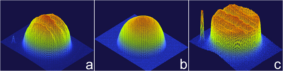
The three 3D pixel intensity plots presented here correspond to the above red-filtered Jupiter raw image a), the elliptical "mask" used to correct limb darkening in this specific image b), and the limb-corrected Jupiter image c). Notice how the "dome-shaped" pattern that exists in plots a) and b) is replaced by a typical "plateau" in the corrected plot c), highlighting the differences between the brighter "zones" and darker "belts" as fairly straight "grooves". Also noteworthy is the higher intensity of Ganymede and the more pronounced background noise in the 3D pixel intensity plot corresponding to the limb-corrected final image c). This results from the fact that, to correct limb darkening, the elliptical "mask" b) was divided from the original raw image a), and the "mask" b) has no signal for the satellite. As a consequence, the pixel intensity along the planetary disk was vastly reduced with respect to the satellite, and became closer to the background noise.
PLATE 5

Click here for a larger image (196kB)
The BMP version of the mask that contains the central artifact a), is opened in Adobe Photoshop and the area surrounding the defect is selected with the "magic wand" tool b). This selected area is then subjected to a Gaussian blur (c); radius=20 pixels). The selection edge is then "hidden" to better show the dynamic range of the blurred selection with respect to the rest of the mask (d); "view" menu, then "show", then uncheck "selection edges"). It is fundamental that the selection edge is just "hidden" and not "deselected". Next it is necessary to modify the gamma of the selected region until it matches the rest of the elliptical mask (e); "image" menu, then "levels"; see also central panel of plate). To further homogenize the interface between the modified and unmodified regions of the mask, a "border" is activated at the location of the selection edge (f); with the edge still "hidden", go to the "select" menu, then "modify", then "border", and choose a value about 10). Gaussian blur the selected border (radius=4 pixels), deselect it to see the result, and save the corrected mask in BMP format g). Several of these masks can be averaged to produce a better quality "master mask" h).
PLATE 6

Click here for a larger image (428kB)
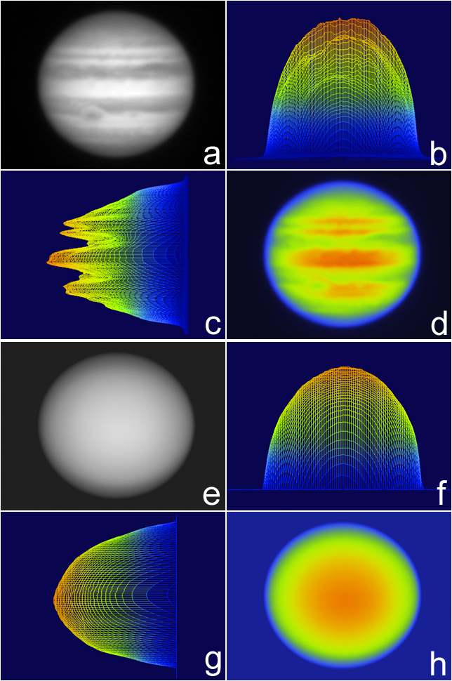
Images a) and d) show the same blue-filtered raw image of Jupiter, only corrected for bias, dark-current and flat-field, visualized in a grayscale and false-color LUT, respectively. Figures b) and c) represent the 3D pixel intensity plots from this blue-filtered raw, prepared to simulate polar and equatorial views, respectively. Notice how the "grooved" profile due to differences between the brighter "zones" and darker "belts" is better visualized in the equatorial view c).The group of the four images e)-h) at the bottom depict the elliptical "mask" prepared to correct the Jupiter image. As above, e) represents a grayscale palette, h) a false-color LUT, and f) and g) represent "polar" and "equatorial" perspectives of the mask, respectively. Notice the resemblance between the planet's and the mask's 3D-plots.
PLATE 7

Click here for a larger image (641kB)
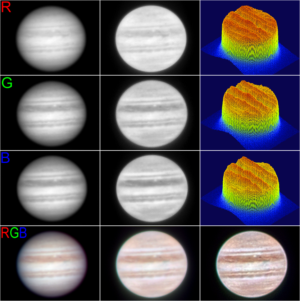
The first three rows of this image represent the red, green and blue channels used to build up a true-color RGB image of Jupiter. At the left are shown raw filtered images, only corrected for bias, dark-current and flat-field. At the center are visualized the same raw images, after correction for limb darkening, and at the right are the respective 3D pixel intensity plots of the corrected images. Notice that limb darkening is more pronounced in red-filtered image than in blue-filtered one. Also notice that the 3D pixel intensity plot obtained from the blue-filtered image exhibits deeper "grooves" that that obtained from the red-filtered image.This is due to the well known fact that the reddish "belts" of Jupiter are much more evident/darker when observed through a blue filter. The last row shows RGB images of Jupiter, produced by merging the three channels just above, obtained before (left) and after (center) limb darkening correction. The third RGB image (right) is just an unsharp-masked version of the corrected image (center). When compared to the original RGB image (left), these two corrected images (center and right) show a reddish hue at both "f" and "p" limbs, interpreted as the result of the more intense limb darkening in the red that is reversed after the correction.
PLATE 8

Click here for a larger image (620kB)
Image a) shows a raw image of Jupiter, obtained with a ultraviolet filter and corrected for bias, dark-current and flat-field.This kind of image, when obtained through small aperture telescopes, is rather noisy even if long integrations are used (30-60secs). For this reason, the image a) was filtered through the "Wavelet" command of IRIS software (see text) and subjected to unsharp-masking prior to limb darkening correction. The result of this processing is shown in b), and the final image after limb-darkening correction is depicted in c). The 3D pixel intensity plots shown in d) and e) correspond to images b) and c), respectively. Notice the characteristic "plateau" in e), with deep "grooves" corresponding to the contrasty "belts", and the noisy pattern surrounding the planetary disk.
PLATE 9

Click here for a larger image (659kB)
Methane-band imaging with small aperture telescopes produces noisy raws containing very low signal levels even when long integrations are used (up to 5mins). In addition, the signal is heavily concentrated around the planet's equatorial and polar regions. Both facts make the direct production of a useable elliptical "mask" for limb darkening correction virtually impossible. In practice, a suitable "mask" can be made from a red- / infrared-filtered image grabbed before or after the methane image. It is important that image scale and camera orientation are maintained, and that a similar date is used so that the planet illumination angle does not change. Image a) shows a red-filtered image corrected for bias, dark-current and flat-field, grabbed the day before the methane image was obtained. The elliptical "mask" produced from this red-filtered image, shown in b), was processed with a Gaussian filter in order to yield the final "mask" c). A methane-band image of Jupiter, corrected for bias, dark-current and flat-field is shown in d).This methane-band image was filtered using the "Wavelet" command of IRIS software to produce the less noisy image e), which was then limb-darkening corrected as shown in f). Notice that the methane-bright polar hoods become much more intense in image f), a south temperate "oval" becomes more evident, and the dark features north of the equatorial "zone" are better visualized. Also interesting is the fact that, although most of the planetary disk exhibits pixel levels close to the background, it is largely noise-free. The issue of background noise enhancement following image division by the elliptical "mask" has already been mentioned earlier.The 3D pixel intensity plots shown in g) and h) correspond to images e) and f), respectively, and confirm what has been said. The almost uniform intensity of the methane-bright equatorial "zone" from limb to limb, shown in h) is evident.
PLATE 10

Click here for a larger image (196kB)
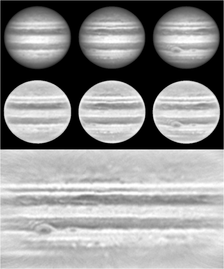
The top row of this plate shows three blue-filtered images of Jupiter obtained in the same night and showing planet rotation.These are single raws, corrected for bias, dark-current and flat-field, and then subjected to mild unsharp-masking and wavelet analysis.The middle row presents these same images following limb darkening correction. On the bottom is seen a grayscale planisphere obtained from the limb corrected images. Using the IRIS planetary cartography module (see detailed instructions in Christian Buil's web page), cylindrical projections were produced and saved in BMP format. Blending of the three cylindrical projections (one projection for each of the images) was performed in Adobe Photoshop. Only very minor adjustments in the "gamma" of the layers were necessary to originate this partial planisphere (only the continuous part is shown), where the image boundaries are virtually invisible. This would not have been possible without limb darkening correction.
PLATE 11

Click here for a larger image (381kB)
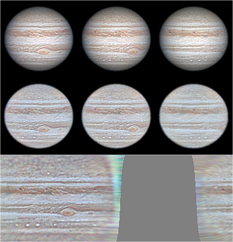
The top row of this plate shows three RGB images of Jupiter obtained in the same night and showing obvious rotation of the planet.These images exhibit plenty of detail because they were obtained under very favorable seeing, and result from averaging and unsharp masking a series of ten raws for each filter.These images had been conventionally processed earlier to produce a data file sent to ALPO, BAA and International Jupiter Watch. I just recovered the RGB originals in TIFF format, split the channels and saved them in BMP format to be read in IRIS.The middle row shows the same images following limb darkening correction, and at the bottom is seen the RGB planisphere obtained from the limb corrected images. Using the IRIS planetary cartography module (see detailed instructions in Christian Buil's web page), cylindrical projections for each filter were produced and saved in BMP format. RGB merging and the blending of the three cylindrical projections (one RGB projection for each of the images) was performed in Adobe PhotoShop. Only very minor adjustments in the "gamma" of the layers were necessary to produce this planisphere, where the image boundaries are virtually invisible. This would not have been possible without limb darkening correction. Notice how a considerable amount of the whole planet's atmosphere is visualized with just three images.
All Images and Texts on these pages are Copyrighted.
It is strictly forbidden to use them (namely for inclusion in other web pages) without the written authorization of the author
© A.Cidadăo (1999-2001)