This article is a full text version of a communication made during the
|
Abstracts
Speckle Interferometry with mid-sized amateur telescope: why not?
This talk shows how using interferometry methods provides routinely accurate measurements with a mid-sized amateur telescope. It is illustrated by the implementation of a homemade 410mm telescope dedicated to double stars measurements and highlights the most important practical tips. The results of a 1000 measurements campaign are briefly discussed.
As a part of the solutions used during this campaign, a focus is made on the new version of Reduc software now including interferometry reduction routines. This version will be released to the public after the meeting.
Interferometría con un telescopio amateur: ¿por qué no?
Esta comunicación muestra cómo los métodos de interferometría permiten la obtención rutinaria de medidas de calidad con un telescopio amateur. Este hecho se ilustra mediante el uso de un instrumento de 410 mm de diámetro dedicado a la medición de estrellas dobles y se resaltan los aspectos prácticos más importantes. Los resultados de una campaña de 1000 medidas son brevemente discutidos.
Como parte de las soluciones utilizadas en el curso de esta campaña, es remarcable la nueva versión del programa Reduc que ahora incluye técnicas de reducción de medidas interferométricas. Esta versión estará disponible públicamente después del meeting.
Introduction
The speckle interferometry is a favorite professional tool for measuring double stars. Some rare amateurs use this technique on missions in observatories, but none seem to use it routinely with a classical amateur instrumentation.
There are two major classes among the instruments used daily by amateurs:
- those whose resolution is mostly limited by the diameter
- those whose resolution is almost always limited by the atmosphere
The border between the two groups obviously depends on viewing conditions, it is usually around 20 to 30 cm in diameter.
When the seeing limits the resolution, the conventional imaging fails to provide measurable images of close pairs. Does the speckle interferometry brings a solution for amateurs as it does on the big professional instruments? The answer is yes. The purpose of this discussion is to share with you a resolutely practical point of view that justifies this response.
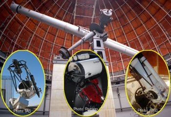 |
Some amateurs involved in speckle interferometry: |
Observatory and Instrument
When I built my 400mm telescope in 2008 to replace the old T200, my goal was to obtain measurements of moderately faint and close double stars (mv ~ 11.12, rho in the range of 1"to 3"). Given the usual conditions on the site, I did not think I would be able to obtain regularly good measures on closer pairs. The observatory is located close a major river and at an altitude of 20 meters, conditions less than ideal for high resolution.
The instrument is a Newtonian telescope, the main mirror has a diameter of 408mm with an optical focal length to 2052.5mm. The minor axis of the secondary mirror is 72.5mm. The first light took advantage of exceptionally calm sky and the telescope showed that observations limited by the diffraction can be achieved.
Obviously it's very different when normal conditions are restored and scintillation, agitation and spreading play their symphony.
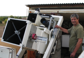 The 408 mm telescope |
First light on COU 407 r=0"4  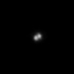 A selection of the best frames 7 img / 600 (1%) |
 Another example with exceptional conditions |
2009: Measures with the Audine Camera
The first camera used on the T400 is an Audine camera shipped with a KAF400 sensor (matrix 768x512, 9 microns square pixels). It is installed behind a Televue 5x optical amplifier, the effective focal length is 11.96 meters.
Using conventional imaging (manual selection of the best images and shift-and-add) measuring couples beyond 1"3 is generally quite easy. With tighter couples we must make a severe sorting in order to find some measurable images. Using the lucky-imaging technique imposes to image at least a thousand frames to have any chance of finding enough correct images. This is a problem with the Audine whose readout rate is low. Getting 1000 images requires 40 minutes! It's enough to discourage the most stubborn observers.
The minimum exposure time set by the shutter of the camera is 60 ms. It's too long to freeze the fast motion of the atmosphere and this further reduces the chances of finding good images. One can speaks of miracle-imaging!
Audine KAF-0400 768x512 9x9m Min exposure=60ms Frame rate=long ! 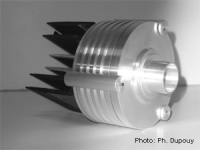 Configuration: F=11960mm E=0"1552/px FOV=2'x1'3 |
 Miracle Imaging on Gamma Virginis |
However 60 ms is fast enough to see a speckled structure blurred by the fastest movements of the atmosphere. These blobs are formed when individual speckles are merging when exposure time is too long. These "super speckles" (the term is borrowed from Christian Buil) carry, however, essential information on the relative position of components.


HU 987 r=1"09, the phenomenon is clearly visible on the animation. Under these conditions and despite the large separation there are only 2% of usable images. The best image of the series is at the center, it is difficult to measure. Right: an autocorrelation image obtained with Reduc. |
It 's during the reduction that the methods of speckle interferometry show several key advantages over conventional imaging:
- Treatment with autocorrelation allows the measurement of images unusable with conventional treatment
- Some hundreds of images are sufficient, typically 200 to 400 for an autocorrelogram. Even with the slow readout rate of the Audine 4 pairs per hour can be visited, enough to give courage again to the observer!
- Sorting images is unnecessary, this saves a considerable amount of time during the reduction and also removes the subjectivity of manual frames sorting
Measurements are possible up to about 0 "6, twice the resolving power of the telescope. Measuring with confidence below this limit requires excellent weather conditions.
|
2010: Measures with an Atik314 Camera
In 2010, the telescope was equipped with an Atik 314L. As the Audine camera, it is very common among amateurs. The sensor has a matrix of 1392x1040 pixels, 6.45x6.45 microns. With the 5x Televue amplifier, the effective focal length of the imaging system is 11.40 meters. This camera appears much better suited to work on double stars:
- Thanks to smaller pixels, the sampling is smaller and the focal length remains reasonable.
- The readout speed is comfortable: 3 to 4 frames / second when defining a window of 128x128 pixels at the center of the sensor.
- The major advantage is the shutter speed. Exposure times are typically 20 ms for stars of magnitude 10 and can be downsized to 1ms on the brightest targets.
With these features, we work more closely to the usual conditions of speckle interferometry. The pictures are better structured and speckles are fine. The performances improve and 70% of the measurements are carried out between 0"3 and 1"5.
Atik314L+ -
ICX285AL 1392x1040 - 6.45x6.45 m Min exposure=1ms Frame rate: (128x128px)=4 fps 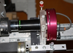 EFL=11400mm E=0"1167/px FOV=2'7x2' |
STT 413  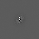 m:4.7/6.2 r=0"9 exp: 1ms 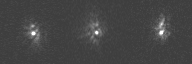 Lucky images: 3/400 ~1% |
HU 940  m:9.2/9.8 r=0"5 exp: 7ms  |
COU 492  m:10.2/10.3 r=0"5 exp: 20ms  |
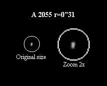
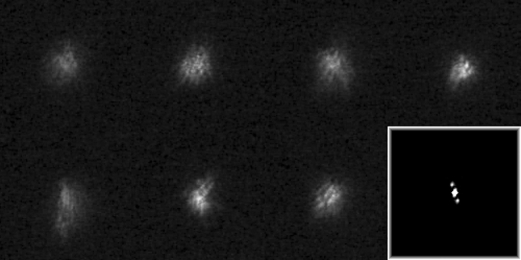
At the limit of resolution power COU1271 mag 9.4/10 r=0"34    Left: the 4 best images |
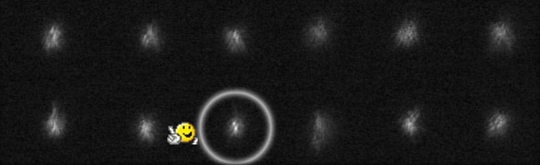
BU 1127 m:7.3/9.2 r=0"75 Audine 60 ms Super-speckles Center : three best images animation Note how the position angle changes    Atik 10ms    |
At the limit of resolution power |


Reductions
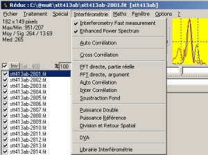 |
All reductions are made with a version of Reduc dedicated to speckle interferometry. It implements the autocorrelation functions, cross-correlation and DVA. The measurements are routinely performed on the autocorrelation image. The ambiguity of 180 ° is solved by creating a cross-correlation image or a composite image when possible. After processing a series of images Reduc provides an autocorrelogram and a series of images that are processed by subtracting a mean mask in order to reveal the peaks. The mask must be adapted according to the optical configuration. With the T400 at F/D=30, the best results are obtained with 3x3 and 5x5 cores. |
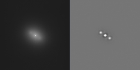
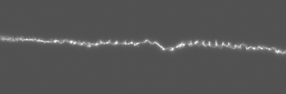
Left: the peaks are hardly visible on the autocorrelogram.
They are clearly identified using a 5x5 mean mask
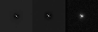
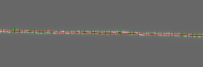
Left: the autocorrelogram used for the measurement.
Center: the difference in intensity of the peaks showed by the cross-correlation* indicates
the orientation of the couple as it is found with conventional imaging at right
(*) the cross-correlation should show the brightest and faintest peaks oriented respectively to the true PA.
Reduc swaps the image in order to put the brightest peak in the quadrant where the secondary is located.
I find this very comfortable when using the one-click measurement feature (see Reduc users manual).
Calibration
The calibration remains the cornerstone of any measurement, it is probably the biggest problem with amateurs instruments. The T400 is on a stable mount and the camera stays in place for several months during the campaigns of observation of double stars. It seemed stronger to make an independent calibration rather than using the traditional method of standard stars.
Sampling:
It is determined in three steps. In the first step the camera is placed at the prime focus and records series of images of several stellar fields containing random pairs of stars of near equal magnitudes, separated by a few arcseconds and oriented in various directions.
During the second step the same fields are imaged using the measurement setup.
Finally, all the couples present on both sets of images are reduced by using a whatsoever sampling value (other than zero!). Each pair has a separation df at prime focus and dm with measurement configuration (ie with the focal amplifier, filters ...). The ratio dm/df provides the scale factor between the two configurations.
By applying this scale factor we deduce the effective focal length of the measurement configuration.
Obviously it works only when the focal length of the prime focus is perfectly known. Take care with commercial telescope and control yourself !
Prime focus 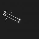 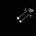 |
Measurement setup 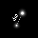 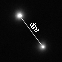 |
EFL = F x dm/df
|
Sampling is calculated with the usual formula and depends only on two physical quantities precisely known (focal length and pixel size). The essential data are summarized in the table below:
Prime focus |
Measurement setup |
||||
Camera |
Focal length |
Sampling |
Effective focal length |
Sampling |
Field of view |
Audine |
2052.5 mm |
0"904/px |
11.96m |
0"1552/px |
2'x1.3' |
Atik 314L |
2052.5 mm |
0"648/px |
11.40m |
0"1167/px |
2.7'x2' |
Orientation:
The east/west axis is determined by the method of stellar trails. The camera and optical train are installed so that the only possible movement is the rectilinear translation needed for focusing. The whole setup remains in place during all the campaign, the calibration is performed over several nights of good seeing. Uncertainty about the direction of the camera is about 0°2.
 |
 Might be difficult to obtain a good calibration tonight. Nevertheless measurements are possible :-) |
Results
The observation campaign was conducted in two phases. The results are summarized in the table below and detailed measures are published in Observations et Travaux #75.
Campaign phase |
Camera |
# Nights |
# Doubles |
Orbital systems |
|
Phase I |
May/December 2009 |
Audine |
75 |
429 |
41 |
Phase II |
February/July 2010 |
Atik |
63 |
579 |
125 |
138 |
1008 |
166 |
Another positive aspect with the use of interferometric techniques: the number of nights observed is greater, about 120 nights / year, it was 80 nights / year before using interferometric techniques.
The bar graphs show the evolution of the observing program.
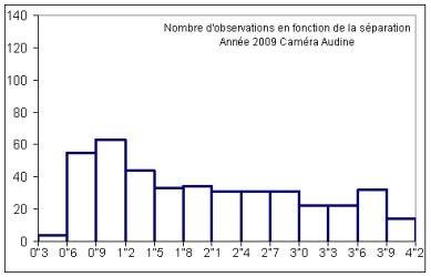 |
During 2009, measurements are initially carried out on a wide range of separations in order to validate the procedures. The reduction with autocorrelation partially overcomes the turbulence. This is the era of "super speckles". With the limits of the equipment the measures below 0"6 are exceptional. |
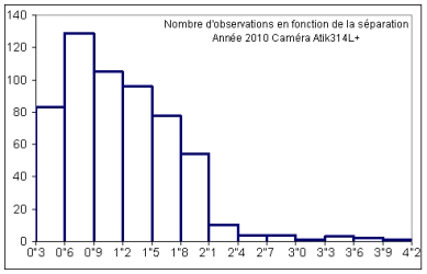 |
By 2010, the equipment is better suited to work with speckle interferometry. The observing program dramatically shifted towards the lower separations. The measures below 0"6 become routine. |
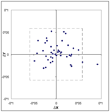 |
Spatial distribution of residuals. Differences (dX, dY) are then brought The average position error is ~ 20 mas.
|
Conclusion
After 140 nights practicing with these methods, I found only favourable arguments, among them:
- The opportunity to observe every clear night without worrying about the seeing
- The optimal use of the instrument
- Measurement accuracy and repeatability
- With the appropriate software the reduction procedures are rapid and objective
About difficulties ... that aren't real cons:
- Finding the right focal length allowing both to separate speckles and to preserve enough light
- Without filtering the speckles lengthen significantly because of atmospheric dispersion when working beyond 25 ° of zenithal distance
- The calibration could be difficult for a mobile setup
What is remarkable is that it is not necessary to use high-end cameras and the latest technology to work routinely at the resolution limit. This is probably the most important lesson I retain from this experience. Amateurs who own a telescope larger than say 12" or 14" sometimes get frustrated of being limited by the atmosphere. The application of speckle interferometry methods will give them the greatest satisfaction!
Bibliography
- Bagnuolo, W.G., 1992, Absolute Quadrant Determinations from Speckle Observations of Binary Stars, AJ Vol. 103
- Buil, C., 1989, Astronomie CCD. Société d'Astronomie Populaire, Toulouse
- Gili, R, Agati, J.L., 2009, Measurements of double stars with the 76 cm refractor of the Côte d’Azur observatory with CCD and EMCCD cameras, Observations & Travaux 73
- Hartkopf, W.I. & Mason, B.D., & Worley, C.E. 2001a, Sixth Catalog of Orbits of Visual Binary Stars
- Hartkopf, W.I., Mason, B.D., Wycoff, G.L., & McAlister, H.A., 2001b, Fourth Catalog of Interferometric Measurements of Binary Stars
- Losse F., Reduc, logiciel de réduction: http://www.astrosurf.com/hfosaf/
- Losse F., 2010, Double Stars Measurements : 2009-2010 Campaign, , Observations & Travaux 75
- Trégon, B., Castets, M., Double stars measurements using speckle interferometry with the t60 at pic du midi observatory, Observations & Travaux. 73
- Turner, N., 2004, Speckle Interferometry for the Amateur in Argyle, B. Observing and Measuring Visual Double Stars, Springer-Verlag
- Turner, N.H., Barry, D.J., & McAlister, H.A., 1992, Astrometric Speckle Interferometry for the Amateur, IAU Colloquium 135, ASP Conference Series, Vol. 32