|
HF
Propagation tutorial
|

|
|
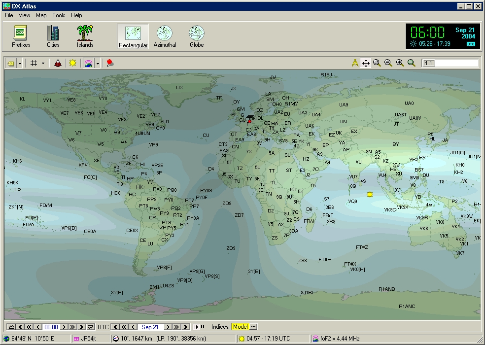
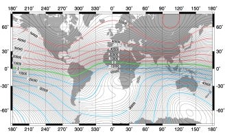
F2-region
critical frequency map showing some "islands of
ionization" along the equatorial region called the
"equatorial anomaly". |
by
Bob Brown, NM7M, Ph.D. from U.C.Berkeley
Down-Sizing of the Ionosphere
(V)
In
the previous page, I showed one sample contour of a global map of the F-region,
for 10 MHz when the SSN was 137. You can go back to the map to see how it spilled over into
the hours of darkness. But that was only one contour. So
the question comes down to the rest of the map, what other contours
were like and their limits in critical frequency.
Looking
at the sample contour, it is easy to think that parts of the globe
closer to the sub-solar point would have higher values of critical
frequency, up to 16-17 MHz. After
all, the sun was more overhead for there and the solar UV had less
atmosphere to penetrate. But
at larger zenith angles, particularly toward the polar regions, the
critical frequencies would be lower, going down to 6-7 MHz. All that for a SSN of
137.
What
about lower SSN, say toward solar minimum? Then, for the region where the critical frequency was 10 MHz
earlier, you can just put in 5-6 MHz and at higher latitudes, you
can put in 3-4 MHz while at low latitudes, the value is 11-12 MHz.
But whatever the SSN, the highest critical frequencies are
always found at the lower latitudes. As a practical matter, that is an explanation why contest
DXpeditions go toward equatorial regions; the bands are always open
there and it is just a matter of how far their signals go poleward
before running out of sufficient ionization.
So
I like to say that the low-latitude regions are the most robust of
the ionosphere. But there is a difference between "robust" and
"ROBUST", say for solar minimum and solar maximum.
Before
getting to that, I should point out there are "islands of
ionization" at low latitudes, as shown by the additional
contours given at right. These islands of strong ionization
develop in the
afternoon/evening local hours. This is called the "equatorial
anomaly" and has profound effects for propagation, giving rise
to long, chordal hops on HF and DX on VHF
Those regions are a regular part of the ionosphere, day in
and day out, and the high level of ionization there adds to the
robustness that I spoke of earlier.
A
few paragraphs earlier, I made mention of the fact that global maps
of the F-region change with solar activity. One way of making these ideas more vivid in one's mind is to
think of them like relief maps, with a "frequency surface"
that rises or falls in height as critical frequencies change with
increasing or decreasing SSN.
|
|
|
N-S
cross-section of the F-region for two different sunspots numbers. |
The
quantitative side of that approach can be shown by means of a N-S
slice through the global maps that one obtains for two different sunspot
numbers as displayed at left, adapted from an original plot from the
PropLab
Pro program.
Those
N-S cuts across the F-region maps show the two "islands"
of the equatorial anomaly as well as the deep notch in between them.
Also, it shows again the geomagnetic control of the
ionosphere by the asymmetry of the ionosphere at 120°E, due to the
fact that the magnetic dip equator is about 5 degrees north of the
geographic equator at that longitude.
Admittedly,
the above graphics are pretty crude but they cover the main aspects
of the ionosphere - E-, F- and F2-region maps - showing how
ionization is distributed and how it varies with changes in solar
activity. It is within those regions that we are trying to propagate
signals.
So we should
lay down some great-circles to see where the paths are going
relative to the ionization. The test, of course, is if the effective vertical frequency along a path
is less than the critical frequency encountered. As long as that's true, propagation will continue; otherwise,
the RF will penetrate the F-region and be lost.
Looking
at the last graphic, you can see that "the test" gets
tougher at high latitudes where the critical frequency is on the low
side, a few MHz. Thus,
there will be angles at which the RF penetrates the ionosphere and
is not returned to ground level. That is "skip",
discovered by John Reinartz back in the mid'20s, and obviously gets
worse at higher frequencies.
In
that regard, there is one "side light" to that on the
higher bands. Thus, it
is quite easy to "pass the test" and work to the south on
21 MHz, for example, as the ionosphere is quite "robust"
in the N-S direction. But
looking at the last figure, one can see that the ionosphere is
"puny" in the E-W direction, with very low critical
frequencies. As a result, when chasing DX on 21 MHz, skip makes it impossible to hear
the station east or west of you that got the South American contact
that you were trying for.
At
this point, our discussion comes down to exploring the aspects of
the distribution of ionization, vertically and horizontally. The
vertical distribution determines how signals are refracted or bent
along a path while the horizontal distribution determines whether a
hop is completed or how long it might be. There are two approaches we can follow, the rigorous one
would be to trace ray paths through a model ionosphere while the
practical one would be to use the model in a propagation program,
looking at the critical frequencies at the two control points on a
path to see what the MUF would be and whether one's RF passes the
test.
Ray-tracing
takes us back to the analogy between the flight of a baseball and RF
across the ionosphere. Mathematically,
the flight of the ball is worked out using Newton' Laws, with
equations of motion in two or three dimensions. You should not be surprised if I tell you that equations of
motion for RF can be worked out, with the ionosphere playing the
role of gravity. So,
like any baseball or even spacecraft, the methods of mechanics work
with RF and the equations of motion solved, step by step, to find
the path of RF. In that regard, the PropLab Pro program is
outstanding; all you have to do is put in the locations of the
terminii, the date and time as well as the sunspot number, and it
solves those equations of motion and traces out the path of the RF. Just fantastic!
But
there is one more thing to add; PropLab Pro also includes the role
of the geomagnetic field in the equations of motion. At the upper end of the HF spectrum, that is not important as
the QRG is large compared to the electron gyro-frequency about the
field lines. But down
around 160 meters, the 1 MHz gyro-frequency is comparable to 1.8 MHz
and the effects of the magnetic field no longer appear to be
negligible in the equations of motion. There are some interesting consequences for wave polarization
as well as signal absorption. In addition, signals can get trapped in that valley above the
night-time E-region and ducted to great distances with low loss. But we'll get to that later; first, MUF programs.
 |
 |
|
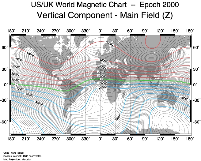
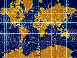
At
left, the intensity of the vertical component of the
world main geomagnetic field correlated at right with
the electron gyro-frequency map created with PropLab
Pro for AM bands from 630 to 1630 kHz and of course with the 160
m ham band. |
|
Note
by LX4SKY. The correlation between the geomagnetic field and
the electron gyro-frequency (EGF) explains the propagation of the
lowest band. This correlation requests some
explanations. EGF is a measure of the interaction between electrons
present in the Earth atmosphere and the vertical component of the
geomagnetic field (Z-field). The closer a transmitted AM or SSB
frequency is to the electron gyro-frequency, the more energy is
absorbed by the gyro electrons from that carrier wave frequency.
This phenomenon mainly occurs with AM signals traveling
perpendicular to the geomagnetic field (especially along high
latitude NW and NE propagation paths). This kind of absorption is
always present and cannot be avoided.
Reference
Notes
Originals
of all the figures mentioned above can be found in my article,
"On the Down-Sizing of the Ionosphere", that appeared in
the July/August '94 issue of The
DX Magazine. Also, the two main F-region maps are on p. 29 of my book on
long-path propagation and also found in Davies' book, Ionospheric
Radio (IEE Electromagnetic Waves Series, Vol. 31).
In
addition, there are a number of ray traces shown in my Little Pistol
book, illustrating skip and showing how RF hops vary with frequency
as well as radiation angle.
Performance
of ionospheric models
Now
we are in a position to talk about propagation predictions. I say that as you understand that predictions require some
sort of representation of ionospheric maps, both E- and F-regions,
and a method that looks at how effective vertical frequencies
compare with critical frequencies along a great-circle path.
I
must admit that I have injected "effective vertical
frequency" (EVF) into the discussion; you normally don't see
that term when you read about propagation. In McNamara's book, Radio
Amateurs Guide to the Ionosphere, he uses another form, "equivalent
vertical incidence frequency", in his discussion but I find
that just too wordy and besides, my choice of EVF fits the bill and
tells the story. I hope
you agree.
Anyway,
we know the test which our RF undergoes as it ascends after launch:
if its effective vertical frequency is less than the local critical
frequency, it will be contained by the ionosphere and if not, it
will go past the F-layer peak and be lost. The propagation prediction business has to do with how that
test is carried out - to what approximation or detail the test is
made and with what sort of model of the ionosphere.
|
|
|
Ham
CAP
propagation map for the 17-m band. Created by VE3NEA it is interfaced with
VOACAP, and with DXAtlas in option. |
I've
already mentioned the control point method in which the test is made
at the first and last hops on a path. That method was developed back in WW-II, by Smith in the USA
and Tremellen in the UK, and was based on the notion that if a path
failed, it was usually at one end or the other.
I pointed out that works well as long as any hops in the
middle of the path do not have LOWER critical frequencies. Beyond that, you should remember that the method represented
a great step forward at the time, even though it was when
ionospheric mapping was in its infancy.
So
the control point method was based on an approximation and its use
involved a database which was both limited and uncertain, at least
at the outset. Nowadays,
the database has improved quite a bit but still will undergo some
revisions in the future as the Internation Reference Ionosphere is
updated from time to time. Today
the standard IRI model is the release IRI-2001.
I
really don't know the details of the first uses of the control point
method but I am familiar with some at the present time. For example, the pioneer program in amateur radio circles was
MINIMUF
from NOAA, with source code first published in QST in December '82. That method used M-factors, numbers between 3 and 4, for
division of the QRG to obtain EVF for comparison with critical
frequencies at about 2,000 km from the ends of the path; for that,
MINIMUF used a database founded on oblique ionospheric sounding.
One
can fault the source code of MINIMUF for not taking into account the
earth's field, leaving out the equatorial anomaly and organizing the
ionosphere only with geographic coordinates. Beyond that, the
database was rather limited in scope. But MINIMUF caught the imagination of the amateur radio
community and all sorts of accessories were attached to MINIMUF,
ionospheric absorption and man-made noise, to mention just a few.
MINIMUF's
shortcomings, the lack of geomagnetic control in the method and no
consideration of radiation angle, placed it in a poor position to
compete with other programs that came along and corrected those
deficiencies. Here, I
have in mind the work of Raymond Fricker of the BBC External
Services. In the mid-80s, he published programs like MICROMUF and MAXIMUF which
included the role of the geomagnetic field and put in radiation
angles so one could compare MUF predictions for more than just the
lowest mode. MICROMUF exists also in Pascal
and an interactive
web form has been developed by Pete Costello for Unix.
|
|
|
Propagation
Prediction, aka PP, by DL6RAI
taking advantage of FTZMUF2. |
Somewhat
later, the german club FTZ Darmstadt introduced a program name
FTZMUF2.DAT, that used a grid
point method to obtain critical frequencies from the CCIR database
and used interpolation to obtain the spatial and temporal data for
making predictions. They
went on to show that FTZMUF2 gave a better representation of the
CCIR-Atlas data for 3000 km MUFs than did MINIMUF. Beyond that, they incorporated FTZMUF2 in their own MUF
prediction program, MINIFTZ4.
Note
by LX4SKY. Four years later, in 1991, Bernhard Büttner,
DL6RAI, also used FTZMUF2 in his own applicated named
Propagation Prediction, PP.
This is one of the first DOS application to display MUF and
other signal strength in a colored line graph as displayed at left.
Then in 1994 Cedric Baechleris, HB9HFN, released HAMFTZ
based on the same grid point method.
But
Fricker used an entirely different approach when it came to the
database for his calculations; he used mathematical functions to
simulate the CCIR database, now in the International Reference
Ionosphere. Then he
used the functions to calculate foF2 at the midpoints of the first
and last hops in his programs, MICROMUF 2+ and MAXIMUF, as in the
control point method.
Those
were the propagation prediction programs available until
the IONCAP
program developed in the late '70s by
George Lane from VOA then by Teters and al. for NTIA/ITS was brought down to a smaller size where it could be
incorporated in home computers. Unlike
IONPRED, which Fricker's method was based only on
F-region considerations - but that gave accurate results in its
limitations - IONCAP deals with fluctuations of signal
strength, it uses a D-region factor, and takes into account man-made noise.
Today the only application always maintained and using a reduced set
of IONCAP functions is PropView from DXLab
suites.
Note
by LX4SKY. In
1985, pressed by the broadcasters' interest, George Lane improved
the IONCAP
model, corrected some algorithms, added new functions, and after
years of research and development created the famous VOACAP
that was released free of right in 1993.
Today VOACAP is considered as the best
ionospheric model, the standard
for comparison.
 |
 |
|
At
left the Windows 32-bit VOACAP
interface, at right ICEPAC.
Both use a improved version of the IONCAP
model rather than the
International Reference Ionosphere (IRI).
From IRI model has been derivated various smaller models to name electron density
models, electron temperature models, auroral
precipitation and conductivity models, F2-peak models,
etc. IONCAP has also been improved and was
incorporated in VOACAP (1985) and ICEPAC
(1993) and "borrowed" by commercial products
like ACE-HF Pro (2001) or WinCAP (2003) prediction models to
name a few. The IRI model is used by very few software
accessible to amateurs, to name PropLab Pro from the Solar Terrestrial
Dispatch and DXAtlas
(2004). |
|
Then
came series of programs, some as accurate as the VOACAP model
for Windows 16 and 32-bit plateforms. Most of them used the new
functions devised by Raymond Fricker and other scientists or
directly the VOACAP engine without additional algorithms.
In
any event, the upshot of the comparisons, is today that Raymond Fricker's programs
and the improvements made by George lane are close in
agreement with
the International Reference
Ionosphere (IRI), then came
all non-VOACAP-based applications that give a rough estimation of
propagation conditions, and far behind all DOS executable like MINIFTZ4
and other MINIMUF considered as the poorest and displaying often
very few information.
But
how well the
underlying VOACAP database matches the real ionosphere (e.g. CODE
GIM model) compared with
IRI, the best representation available at the present
time ?
Real-time
status of the ionosphere
from GNSS Group, Belgium
Software
: CODE
GIM model
In
that connection, I undertook a study of how the mathematical F-layer
algorithm in Fricker's MAXIMUF compared with IRI, not just for a
path or two but over the entire world. Thus, foF2 values were calculated at intervals of 5° in
latitude and 5° in longitude from Fricker's mathematical functions
and compared with corresponding values from IRI. That method showed where Fricker's values were low, where
high and an overall measure of his methods.
The
result was that Fricker's method, when used to make a map of the
F-region, gave good agreement over the entire globe with the values
from IRI, point by point, but the agreement could even be improved
considerably by the simple offset of 1 MHz added to the foF2 values
calculated by his methods.
|
|
|
SNR
calculated with VOACAP for a circuit between UA3 (Moscow)
and ON (Wépion) on August 5, 2004 at 2200 UTC for 100 W
output (SSN = 27, SFI = 85). VOACAP predicts a signal
strength in Belgium of -140 dBW or S3 and a S/N ratio of 27
dB, thus quite weak. Figures matched signal reports given on
the air. |
Put
another way, Fricker's foF2 map was very much like the map from IRI,
with details such as the islands of ionization showing up as well as
various aspects of geomagnetic control, but the critical frequencies
were a bit low. All in all, I found it amazing!
And
that approach proves to be just another way of testing F-layer
algorithms, seeing if they can make a good ionospheric map or not.
MINIFTZ4's algorithm gets good marks in that regard but with
problems from its interpolation methods while MINIMUF's F-region map
has little resemblance to a real ionosphere on a global scale. That
accounts for some of its erratic predictions for DXing.
Unfortunately,
when I made my tests
the F-layer algorithm of IONCAP was not available, so comparisons with
the IRI remain to be done with VOACAP which sources are available
from NTIA/ITS. Perhaps some of the VOACAP developers
will do that in the future. But
whatever the outcome, VOACAP is always the best HF propagation program and
provides some of the other aspects of propagation prediction that
are important. Thus, in addition to having methods for calculating
MUF, LUF and other HPF, it deals with the range of values of critical frequencies
resulting from the statistical variations in the sounding data.
Here,
I refer to statistical terms like the median as well as the upper
and lower decile values of critical frequencies from the sounding
data. In a propagation
setting, the median value of the data at a particular hour during a
month would be one such that half the observed values lie above it
and half fall below it. If a median value is used in propagation calculations, one
obtains what is termed the Maximum Useable Frequency (MUF) for the
path. The upper and lower decile values of critical frequency have
to do with the 90% and 10% limits. Thus, the upper decile value during a month of observation is
a frequency which is exceeded only 10% of the time, 3 days, while
the lower decile value during a month is a frequency which is
exceeded 90% of the time, 27 days.
When
those values are used in propagation calculations, one then obtains
the Highest Possible Frequency (HPF) and the Frequency of Optimum
Transmission (FOT) for the path. A sample of that kind of calculation is given below (in MHz),
for a path from Boulder, CO to St. Louis, MO in the month of January
and when the SSN is 100 :
|
GMT
FOT MUF
HPF
GMT FOT MUF
HPF
|
|
1
10.7
13.6 17.4
13 6.4
7.5 8.4
3
7.4
9.6 12.0
15 13.0
15.3 17.1
5
5.7 6.9
8.7
17 16.6
19.3 22.0
7
6.1
7.4 9.7
19 18.1
21.1
24.0
9
6.5 8.0
9.4
21 17.7
20.6 23.5
11 5.0 6.1
7.2
23 15.9
18.5
21.1
|
|
Looking
at those numbers, you can see that the HPF and FOT values lie about
15% above and below the MUF values. That should put you on notice; if the propagation program you
use gives only MUF values, the real-time values for the ionosphere
could differ by as much as +/-15%. And that is only from the statistical variations in the basic
data; there are still the approximations in the method to worry
about as well as geophysical disturbances.
But
those remarks apply mainly to the higher HF bands; down on 80 and
160 meters, ionization is not a concern on oblique paths. Instead,
noise and ionospheric absorption limit what can be done. And
propagation programs are useless for those bands as the main
criterion is darkness along paths, not MUFs. But the role of the geomagnetic field is important and
affects the modes that are possible. All that in due time.
As
for geophysical disturbances, those will be our main effort in next
chapter and need not concern us at this point. We are really concentrating on the undisturbed ionosphere and
its properties or modes, variable though they may be. And while still talking about the
VOACAP program, it is
worthwhile to note that its methods deal not only with the
statistics of F-layer ionization, through MUFs and the like, but
also down lower where absorption and noise become have their origin.
So VOACAP has F-region methods which give not only the
availability of a path, the fraction of days in a month it is open
on a given frequency, but also D-region methods which give the
reliability of a mode, the fraction of time the signal/noise ratio
exceeds the minimum required for the mode.
This
was not meant to be something just in praise of VOACAP but for me it
is the best HF propagation analysis and prediction program that I have at my
disposal in a point-to-point prediction perspective. True, there are other programs based on it and you will have
to judge for yourself whether those programs meet your requirements
or not. You should read the reviews out there, on this
website, in QST and
The DX Magazine, to get a feeling for what they can offer you in your
pursuit of DX. If
possible, check with a user to see if the program matches your goals
or needs for DXing.
At
this point, we've come to where ionospheric disturbances from the
impact of the solar wind on the magnetosphere are of real importance.
Needless to
say, they add to the uncertainties that have been cited above. But in contrast to the statistical side of propagation, there
are clues that help deal with the geophysical side of propagation. That will be our task in
the next pages.
Next
chapter
Propagation
modes and DXing
|