|
What
can we expect from a HF propagation model ?
|
|
|
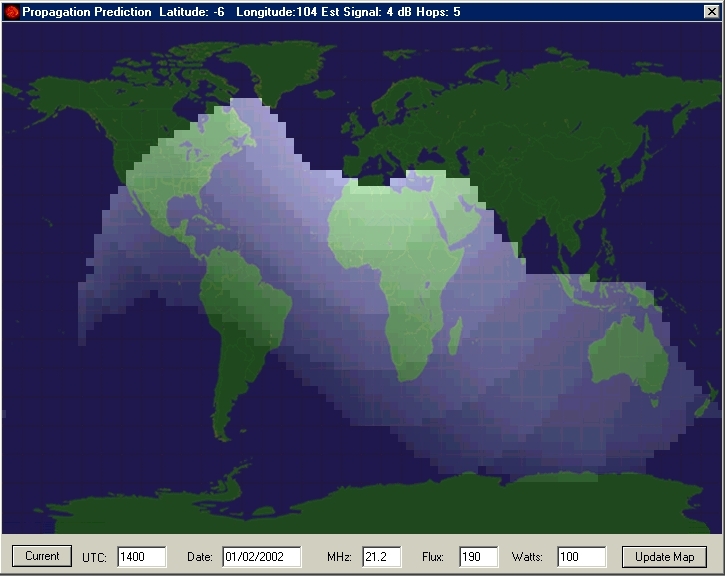
Propagation
forecast generated by DX
ToolBox for the 15-m band on February 1, 2002 at 1400 UTC. |
Simulate
the ionospheric propagation (I)
What can we expect from a propagation prediction program ? What is the objective
of such a program ? What are mandatory parameters to calculate a propagation
prediction with more or less accuracy or reliability ? What are the
most useful charts to estimate an opening toward a DX country ? Here are some
among the many questions at which we will answer to help you selecting your
propagation prediction program.
In
saying this, that means that you have the choice between not only
several applications but that each of them shows probably more or less
features and accuracy. To answer to this question we must thus extend
your scope and come back to the origins of these
applications to see what geophysicists expected from the original programs,
how they have improved them, and with what degree of accuracy and
reliability.
Models
An
ionospheric model is synonymous of numeric forecast. This forecast is
qualified of "numeric" because the state of the ionosphere is
described by series of numbers and physic laws by operations on these
numbers, the whole being processed by supercomputers.
The
method of forecast consists in representing the ionosphere evolution by a
set of basic physic laws, functions that try to represent at best some
specified dynamic processes that develop in the ionosphere.
When
we speak of radio propagation we have to consider all interactions
between the Sun surface and that of of Earth. This "working
space" includes the sun model, the space weather model, and the
ionospheric model without to speak about the atmospheric model that
can be useful to understand the propagation on the top band of 160
meter. Often these master models work with smaller models dedicated
to a specific process or covering only a small location, the master
handling the global computations at large scale and data exchange
between models.
|
|
|
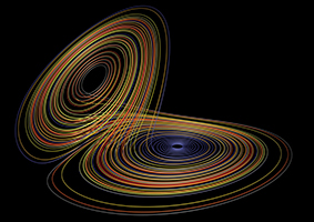
At
left, like in meteorology where the atmosphere is cut
is slices more or less extended and thick depending on
the available data and the required accuracy, a
perfect ionospheric model could also divide the
ionosphere in small volumes in which each variable and
its interactions are processed, then injected in the
international ionospheric reference model in which
will appear small ionization islands and large scale
interactions, all we need to get an accurate forecast.
This model is under development and operational, it is
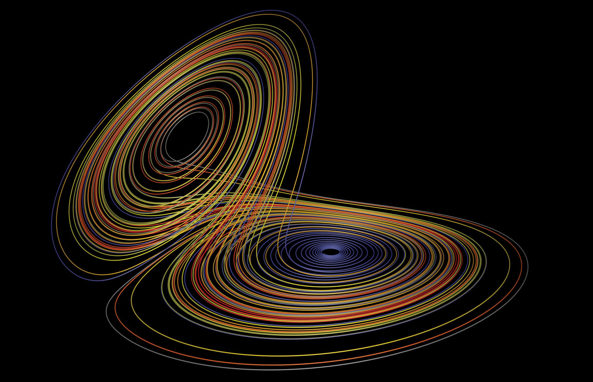
called IRI. At right, a Lorentz's strange attractor, or
how a small "thermodynamic butterfly" can
affect a global system... Like Murphy's Law, the
butterfly effect is never far away to refute your
obervations. Documents Météo-France and
Paul Bourke. |
|
Up
to now, these three or four models exist at various scales but do
not exchange their data. It is even inthinkable to develop a super
meta big "sun-earth plasma model" taking into account all
solar, space weather, geomagnetic, geophysical and weather
conditions, all the less that additional models will be proprably
added to the code to improve its accuracy. These "add-ons"
can be as numerous as Windows fixes, Hi ! The reason is obvious, too many variables
are to be considered in the three dimensions. Worst, they are
interdependent, variables interact each others applying in force the
laws of thermodynamics, including the famous "butterfly
effect" : a small variation in the initial conditions will
amplify with time, transforming for example the simple electron
rotation in a huge malstroem some months later. Hard in these
conditions to forecast anything with accuracy over some times
without to get erratic results.
In
the field that means that today we cannot inject all data in this
"black box" with the hope to get in output a complete
prediction covering any communication circuit and any coverage. But
maybe after tomorrow, if someone if smart enough to develop this
interface and pay for this supercomputer which blueprint does no
exist yet, Hi !
Constrained
by our limited mind and the size of computers (memory, disk space,
CPU speed), we must thus reduce our scope and only inject in our model
a representative amount of data of the real conditions, what represent
already a long list of parameters that we are going to
review. The IRI model 2001 is rather performing and it has
permitted to derive some well-known models dealing with a specific
process or variable like the electron density model, electron
temperature model, auroral precipitation and conductivity model,
F2-peak model, CCIR noise model, etc, each of them including other
models constituted of tens of functions. Here we are in an
environment far from the ham shack : our colleagues are
mathematicians, statisticians and engineers and prefer to compute
differential equations than working on the air, Hi !
Why
simulate HF transmissions ?
Scientists want to simulate HF transmissions to better understand the
behaviour of the ionosphere and effects of radio propagation on communication
circuits that can be two remote radio stations sometimes separated by an ocean
or by the night. Thanks to supercomputers, simulation programs have been quickly
able to show propagation effects with a great accuracy in 2D or 3D.
|
|
|
A
side-view of propagation paths of sky waves at a frequency
of 12.45 MHz for elevation angles from 5 to 50°. The dashed
line indicates the electron density profile. Documents
realized by Andreas
Schiffler on a home computer using a ray tracing program
solving a set of differential equations. |
Today, in fact since the '70s
and the pioneer works of the broadcasting company the Voice of America, these
programs have been down-sized and are available for PCs. Thanks to these tools,
a novice can easily
understand what happens above his head in running simply a propagation
program. At the remark of his correspondent, "you know, this blooming low
band is closing down again... I don't really understand why !", he could
for example very soon answer him "indeed, this happens because the LUF is
raising to this frequency and the D-layer absorbs too much shortwaves. That will
last half an hour then the band will be as clear as this night with stronger
signals". With this knowledge this amateur will be quickly consecrated
"propagation guru" among his friends, Hi !
These simulation tools give
indeed the amateur the opportunity to foresee in a few keystrokes the propagation for any future date, to
review previous propagation conditions or to compare different working
conditions to improve his or her knowledges in this matter.
These programs offer a great interest for contesters and DXers too because they
permit them to plan in advance the best bands to work depending on time of the day and the frequency.
We will come back of this use.
A good simulation program also permits
the ham operator to see how different equipments affect his or her signal
strength at the receive location or the radiation coverage across lands and
oceans. You can also use such programs before buying a new antenna for example,
to simulate effects on transmission coverage of a beam vs. a vertical. But often
these features are not available in the simplest programs.
Once you are used to play with
these applications, from a first sight complex, these programs appear eventually
to be much simpler than expected and also fun
to work with if you are looking for accurate predictions. Funny ? That right,
because as soon as you put the finger on the right variable(s) that affected
your signal, you improve in the same time your knowledge of the ionosphere
behaviour under specific conditions, and it will no more look to an
"ionospherica incognita" as it still looks like to in the mind of most
amateurs.
But more interesting, in
working with a propagation program you do no more loose your time in calling
"CQ DX" in a dead band and thus you learn to work smarter on the air in
appreciating still better your hobby.
Propagation
programs for radio amateurs
For
years astronomers of the visible or unvisible univers (so-called
white light and radio) are monitoring the sun activity, recording
day after day the sun conditions, the number of sunspots, the
occurence of sunflares, prominences, CMEs, properties of the solar wind, and other
cataclysmic event to better understand the sun dynamic and improve
the accuracy models. In parallel geophysicists are checking the status of
the geomagnetic field and the atmosphere, geomagnetic disturbances
and other physico-chemical alteration affecting the ionosphere and
the upper layers of the atmosphere.
Thanks
to satellites orbiting earth, antenna dishes, servers, repeaters and Internet relaying data
between observation sites and observatories, today
these readings are automatic checked by triggering procedures that
immediately warn the concerned people when the sun or the
geomagnetic activity reaches a threshold. These activity reports are
then displayed in charts are released several times per day to the
scientific community and the public.
Unfortunately, ham magazines
being published monthly, data are already almost obsolete when you
read them or give you only a rough estimation of the conditions to
come; the K-index is a short-term forecast valid 3 hours only
and the median A-index value is updated daily. So if you trust in
these tables you could never get an accurate propagation forecast or
discover an opening, just there, in the 20m band in two hours or
tomorrow morning.
In
the U.S.A., to get a forecast faster you can also rely on messages transmitted ny
NIST on the air on WWV frequencies (e.g. 2.5, 5, 10, 15 and 20 MHz on week
days) each 18 and 45 minutes past the hour. Here is a recording
of the WWV signal of 10 kW emitted at 09:00 GMT at 5 MHz. If you
heard it, you have chance to fine tune your forecasts.
Since
the launch of the first satellite in 1957 and the use of
computers, over the years the amount and quality of data collected by
professionals have much improved. Thanks to all these online and updated data,
they have created better quantitative and analytical models of the ionopshere
than in the past, say before the '80s.
Aha
? will tell the amateur, rising suddenly his nose from his WWV
predictions... This interest from the ham community for radio
propagation programs leads us to review whether or not amateur
propagation programs are capable to provide accurate forecasts from this wide variety of inputs.
History
of amateur propagation programs
Historically,
how all this began ? In 1969, the american Institute for Telecommunication Sciences from the
National Telecommunications and Information Administration (NTIA/ITS)
published a technical report
dealing with algorithms to use to predict long-term HF propagation
conditions. Immediately some smart people, engineers and physicists,
extracted the best elements of this report to develop the kernel of
the future ionospheric model. Some years later, from this information
some amateurs developed their own point-to-point propagation programs,
like Prof. Geoff West's GWPROP
that was released... 17 years later.
This
technical report was is fact the blueprint and grandfather of IONCAP. In 1983,
the first IONCAP
model was developed by Teters and al. from NTIA/ITS, soon replaced by an enhanced version developed
by Voice of America for broadcasting purposes, and know as the VOACAP
model or engine. The product is always under development, except that
today fund are no more available but always accepted. The product is thus only supported on email basis.
From 1982
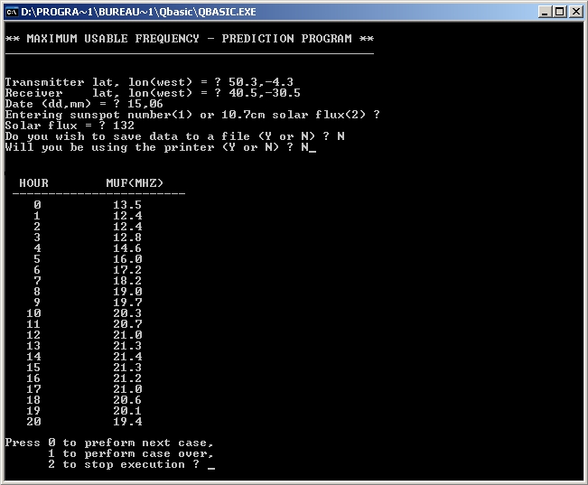
amateurs have had the opportunity to use the first DOS programs like MiniMUF from
NOAA, that evolved to MicroMUF. On its side at
the same time MiniProp was very appreciated too because it was much
easier to use than a product like DXAID for example. Based on the
F-region method used by Fricker in his IONPRED model, MiniProp evolved
to MiniProp Plus that displayed the gray-line and an approximate auroral
oval (it didn't use a K-index function like DXAID), until W6ELProp
was developed for the first Windows environments.
In
parallel, in the late '70s the International Reference Ionosphere, IRI, was down-sized to
run on the first IBM microcomputers. In the years '90s the most well-know program using this PC
version was DXAID
by Peter Oldfield, soon copied but never equaled. It
was probably the best HF propagation program
developed for amateurs. Already at that time it took into account
the solar and geomagnetic conditions and thanks to accurate
functions was able to forecast the auroral oval and any DX
propagation at short-terms. Today only DXAtlas
and similar products reach this quality.
|

|
|
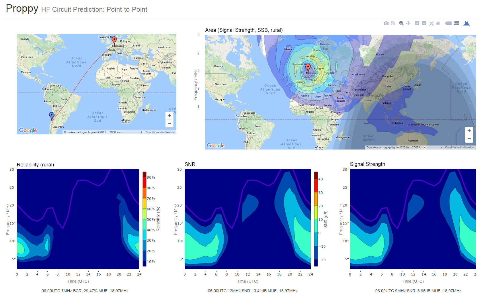
Propagation forecasts calculated with
Proppy
released in 2016 by James Watson (M0DNS/HZ1JW), for a
point-to-point link between LX and CE on August 2016 for an isotropic antenna
and 100 W in SSB. The area prediction is also calculated (the
world map above right). |
Today, following the hardware evolution and specially the performances of
new chips, some of these programs have improved their algorithms and graphic user interface,
they include much more functions and some are
interfaced or exchange their data with other products or even with
telecommunication devices when they are used by the U.S. Government.
As listed in my review of propagation
analysis and prediction programs, these programs counts by tens and have been developed for
most operating systems from Windows to Mac OS and Linux.
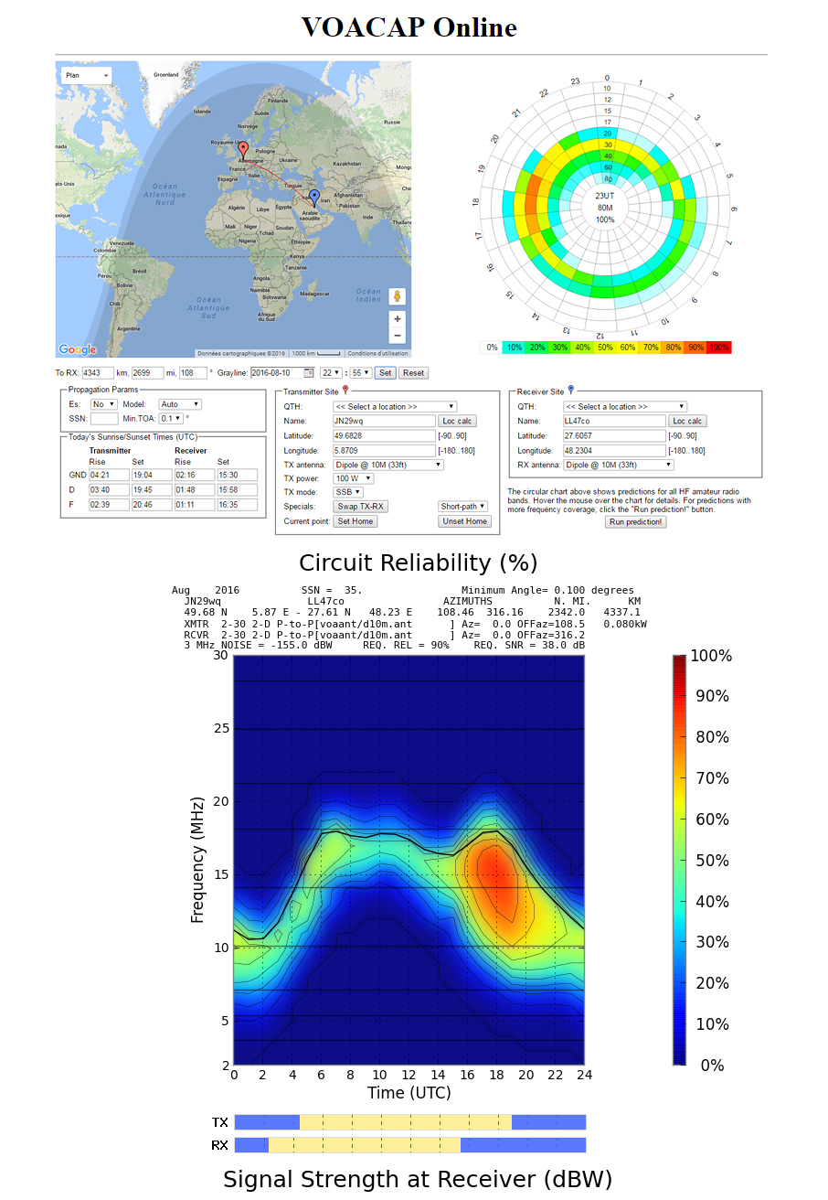
Today VOACAP
is available in two versions : one to install locally on a computer
running under Windows, Mac OS X or Linux, and an online version
a bit lighter available since 2010. Both versions are always very
appreciate by the ham community, military and broadcast stations.
At
last, in 2016 James Watson (M0DNS/HZ1JW), responsible
for porting the VOACAP Fortran
code from the Salford to the GCC
compiler developped Proppy. The name is derived from "Propagation Python"
(Proppy). Using a web interface similar to VOACAP Online but simpler, it differs
from this latter by using the ITURHFProp prediction model (formely REC533) to
calculate performances of HF circuits in accordance with Recommendation
ITU-R P.533-13)
provided by the ITU. The P.533 library is thus a separate application to
VOACAP but unlike VOACAP, P.533 is well documented and actively maintained
by a professionnal body. The ITRHFProp codebase is currently closed source
although comprehensive details of the algorithm are available on ITU website.
Proppy is thus an alternative to VOACAP.
Unfortunately most of
these programs take into account only one parameter, the smoothed sunspot number (SSN) or
its equivalent, the solar flux (SFI). Very few, say less than 20%,
use values of the geomagnetic field (Ap and Kp) considered as
"useless". But it must be known that magneto-ionic effects
become important on 160 meters, where the frequency (about 1.8 MHz) is
close to the gyro-frequency of ionospheric electrons. Atmospheric
noise and weather conditions also affect much the top band. In
addition, the K-index affects the propagation near polar caps and is
thus a parameter that developers must take into account to get
accurate resultats in all working conditions that might experiment
amateurs.
Some
programs use these parameters but often with approximative algorithms
(K-function) instead of interpolating real-time data. Others, say 25% of
applications simply ignore the working conditions like the transmitter
properties (mode used or sometime the power), the antenna specifications (gain,
takeoff angle, bearing), the noise and interference level at target location,
the ground quality (conductivity, dielectric constant)
and even the circuit reliability to name several
parameters that affect the signal quality.
Input
parameters and forecasts validity
|
|
|
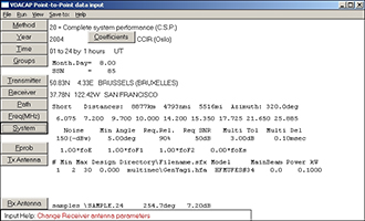
VOACAP
(locally executable version) input screen. Not less than 26 inputs are necessary to calculate
a prediction. Other programs use still more data, sometimes
updated in real-time. |
Why
using so many parameters, do you ask me ? Are these additional
parameters really useful ? Well, all depends on your needs but you
will understand easily that the more data you consider the more complete will
be the model and the probability to get an accurate forecast, that
it concerns an overview at earth scale or a specific communication
circuit between two stations.
Of course parameters by themselves do
not tell all the story, especially if they are injected in a model
using poor and approximate algorithms. It is by far better to use a model
using few functions but very accurate, and focus on a single output
parameter, than using many data injected in approximative models. In the same way
it is better to inject real-time data in functions than median values
that do not allow to calculate a real-time prediction, if not
with a large uncertainty.
Few
publishers have understood the meaning of these trivial remarks. Therefore
you will find many differences (small or much more important) in
results displayed by applications. Here for example, the propagation
map displays a S/N ratio at the target location of 50 dB while this
other program displays only -10 dB... The difference reaches a 6-factor
! One might as well say that such predictions are
useless if they forecast a close band although it is really wide open
! Better to check yourself on the air in calling CQ DX, HI!...
These
variations mainly occur for short-term predictions or in poor to fair
working conditions (low reliability and S/N, disturbances, propagation
changing, etc). It is indeed obvious that when propagation conditions
are excellent, forecasts are no more used as most bands are open to
milliwatt; conditions experimented yesterday will be, with a little
luck, always valid today and next week. In these excellent conditions,
even used bare foot, a small transceiver connected to a whip antenna
could reach DX stations at the first call, or almost ! But everybody knows
that as soon as you worked during the maximum of the solar cycle. What
amateurs requests are accurate forecasts either whenp ropagation
conditions are changing or for specific working conditions. And in
this context, very few programs are powerful and flexible enough to
give accurate results. But can we really improve this accuracy ? This is the
subject that we are going to deal with in the next chapter.
Next chapter
Performances
and limitations of ionospheric models |