|
What can we expect from a HF propagation model ?
|
|
|
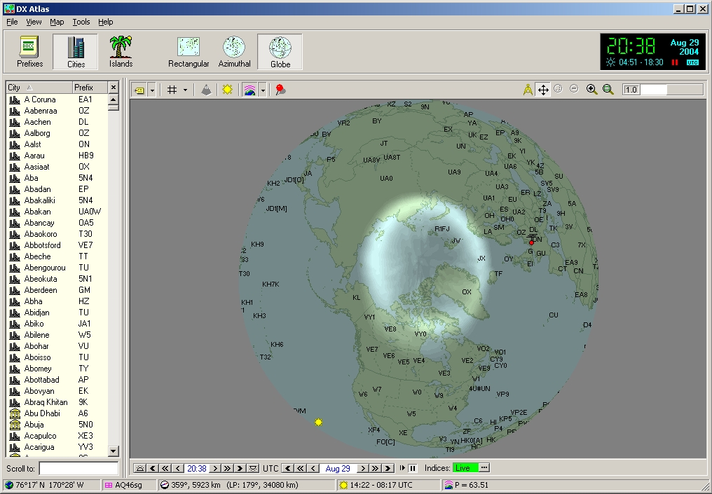
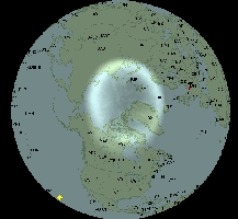
Electron concentration at 320 km of altitude
(F2 layer) as predicted by the CTIP
model at 16:00 UTC.
|
Performances
and limitations of ionospheric models (II)
A
propagation analysis and prediction program establishes its forecasts from statistical analysis
using either empirical or real-time data from which are calculated critical
frequencies, the ionosphere status at global scale or the reliability of the
specified circuit among other parameters.
Empirical
data are based on previous studies made in the field (using ballons or
satellites) which results are stored in data sets (tables or database) or
converted in functions (e.g. polynomial interpolations). Real-time data are
downloaded online from websites receiving in near-real-time data from
ionospheric sounding transmitting by observatories.
Depending
on the accuracy and completness of stored data or functions, and the one of
algorithms used to calculate effects of physico-chemical processes at various
latitudes and heights, one easily understand that statistical analysis will be
more or less complete and accurate.
If
an application works with smoothed values, medians, estimated
monthly or even at longer term (6 months to one year in the case of
sunspot number) that also means that forecasts will be more
optimistic than the ones provided by a more complete model taking
into account the time and additional parameters. If you whish an
optimistic forecast you must select a low reliability (30-50%), and
conversely, select a high reliability (60-90%) to get a more
pessimistic, conservative forecast.
In
spite of these statistical laws, against which nobody can go, some
publishers do not hesitate to pretend that their forecasts are very
accurate using the nec plus ultra model, all solar and geomagnetic
indices, etc. But looking closer their program, such arguments do
not convince for long advanced amateurs. In fact, most of the time
this is unfortunately nothing else that a marketing trick.
Let's
see the different reasons for which an ionospheric model shows, and
will always show inaccuracies.
A.
Utility of Ap and Kp indices
Let's
take an example on the utility of some indices. Several editors
state that their program uses Ap, Kp or Q index, or even the latest
geomagnetic model (storm, etc) to improve the accuracy of their
predictions. But in reality, those publishers do even don't know
what they speak about. Those parameters and not suitable for
automatic updates of the ionospheric model.
In
fact you must know that there is no way of predicting HF propagation
without taking into account the solar and geomagtnetic indices, and all VOACAP-based
applications use both factors. But most of these programs use also median values because so
does VOACAP. There is a good reason for that : the daily and hourly
variations of the ionosphere are huge, and we simply do not have enough data to
estimate these rapid and spatially diverse changes.
 |
|
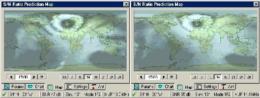
Effect
of Kp index on the S/N ratio (SNR), MUF and TX takeoff angle
estimation at high latitude where geomagnetic effects are the
strongest. Propagation conditions calculated for
the 20 meter band with Ham
CAP for September 2004 using an emitting power of 100 W. At
left forecast for Kp = 9, at right for Kp = 1. The cursor is
pointed on Island (TF). A low K-index increases the MUF of 10% and
the S/N ratio up to 20% at high latitudes. The best takeoff angle
does not change more that 1° in average. So the impact of Kp is
not important but it must be taken into account for all
predictions implying a circuit via high latitudes, say surely
above 50° N and S but its impact is already sensitive in
tropical areas (where the S/N changes of a few dB only). In
addition, without checking Kp you could not predict the auroral
oval, excepting using satellites and ionosondes. |
|
A
good model, I mean accurate even at short term, can predict what happens when the Kp
index increases. Thanks to Kp we know that a geomagnetic disturbance is
developing aloft, but we cannot
tell if it is accompanied by an ionospheric storm or not, and if it
is, then which paths are enhanced and which ones are degraded and to what
extent. It is thus very important to monitor the Kp index and auroral activity,
but only a handful programs deliver accurate and real time
information about the indices and the auroral oval. In fact these
parameters are useless in the automatic propagation prediction because in no
case the Kp input improves a prediction.
To
produce an accurate global ionospheric map (at earth scale), there
is a much better way : it is to use direct, real time ionosonde measurements of the F layer
critical frequency. Instead of trying to guess how Kp influences foF2 (like
NOAA' STORM model
does), we can use the foF2 itself ! DXAtlas
for example, to name a performing and recent application uses such a
feature in tandem with a small application called IonoProbe
to predict the auroral oval as good as SEC
predictions based on NOAA satellites. Recall that Alex
Shovkoplyas, VE3NEA, who developed DXATlas found and fixed an error in
IRI-2001 model, his name being listed in the official IRI source code. DXAtlas
is thus not a propagation model as ordinary as it looks at first
sight...
 |
 |
|
At left, the statistical auroral oval extrapolated
from NOAA-17 satellite data by SEC/NOAA for August 30, 2004 at 20:38 UTC. At right the real-time auroral oval as predicted by Alex
Shovkoplyas, VE3NEA, author of DXAtlas
using real-time ionosonde data and estimated for the same time. DXAtlas prediction is based on the same statistical patterns and real-time
satellite data that the ones used by NOAA to generate their auroral map. |
|
B.
An inherent imprecision
Like weather forecasts based on numerics (models), ionospheric models
will always show an inherent imprecision, IRI-2001 or its down-sized versions
included. Up to date, no model go one step further and fits the IRI model to the actual foF2 values reported by the
ionosonde network. Here also, IonoProbe from VE3NEA does this job and summarizes the real-time data in the effective SSN
value and passes it to DX Atlas, along with other real-time parameters, allowing
the latter to produce real-time maps.
But
is it only possible to increase the accuracy of current models ? We
can collect ionosonde data over long periods of time and perform statistical
analysis on these data. But up to now the picture that has emerged is very
disappointing. In generating a correlogram scientists discovered that the
correlation distance of foF2 is about 2000 km, and the difference of the
measured values from the modeled ones reaches an order of magnitude
That
means that to build an accurate foF2 profile that could be used for ray tracing,
one would need at least a 4000x4000 km grid of evenly distributed ionosondes;
the existing ionosonde network does not even come close to that. Another
approach is trying to use other available ionospheric parameters, such as Kp, Q
index and auroral activity index, to model ionospheric disturbances, and to
estimate the foF2 distribution more accurately.
 |
 |
|
|
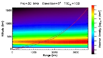
At
left the Signal
Propagation model is a product dedicated to ray-bending. It
takes advantage of VOACAP, Jones-Stephenson, RIBG and EICM
ionospheric models. At right the electron concentration as a
function of the height and latitude as predicted by the CTIP
model. |
|
But
here also, both statistical analysis and a review of available publications have
given very discouraging results. An ionospheric storm for example is a very
complex process that evolves in space and time. To estimate its dynamics, one
would need much more real-time measurements than we can hope to have in the
foreseeable future.
To
get an better view of difficulties that scientists meet with, see for example, the Effects
of geomagnetic storms on the ionosphere and atmosphere paper, a very
interesting document published in 2001 by AGU.
One approach that initially looked very promising was used in the
STORM model developed at NOAA and introduced earlier.
This
model uses the 36-hour history of hourly Ap indices to model the
effect of geomagnetic disturbances on the ionosphere. DXAtlas is the first
amateur program having implemented the STORM algorithm. In addition, VE3NEA
compared his results to AGU predictions, and discovered an error in AGU algorithm as
well. But the striking thing is that the Kp/Ap based corrections that AGU has
published since 2003 were absolutely wrong, and no one have ever noticed this !
Using
Kp in some VOACAP-based application is a first attempt to catch the first order dependency between the geomagnetic activity
and the depletion of the F2 layer. However, in DXAtlas documentation it is clearly stated
that this option is experimental; it was added just to see if there is any
improvement in the predictions due to an ad-hoc correction for geomagnetic
activity. Today, we can conclude that it does not seem to improve the
accuracy of predictions, a conclusion that some people expected for a while.
C.
New improvements
However,
there is a good news. When benchmarking VOACAP and
Proppy
against the D1
databank, Proppy is more accurate as it uses an entirely different method of prediction.
The D1 dataset is an industry standard for evaluating propagation
prediction applications based on ITU-R P.1148-1
describing how prediction tools may be compared in a systematic
manner. Using this method, the standard deviation of error when predicting values with
VOACAP is 19 dB, P.533 reports a 10 dB improvement in the error.
 |
 |
|
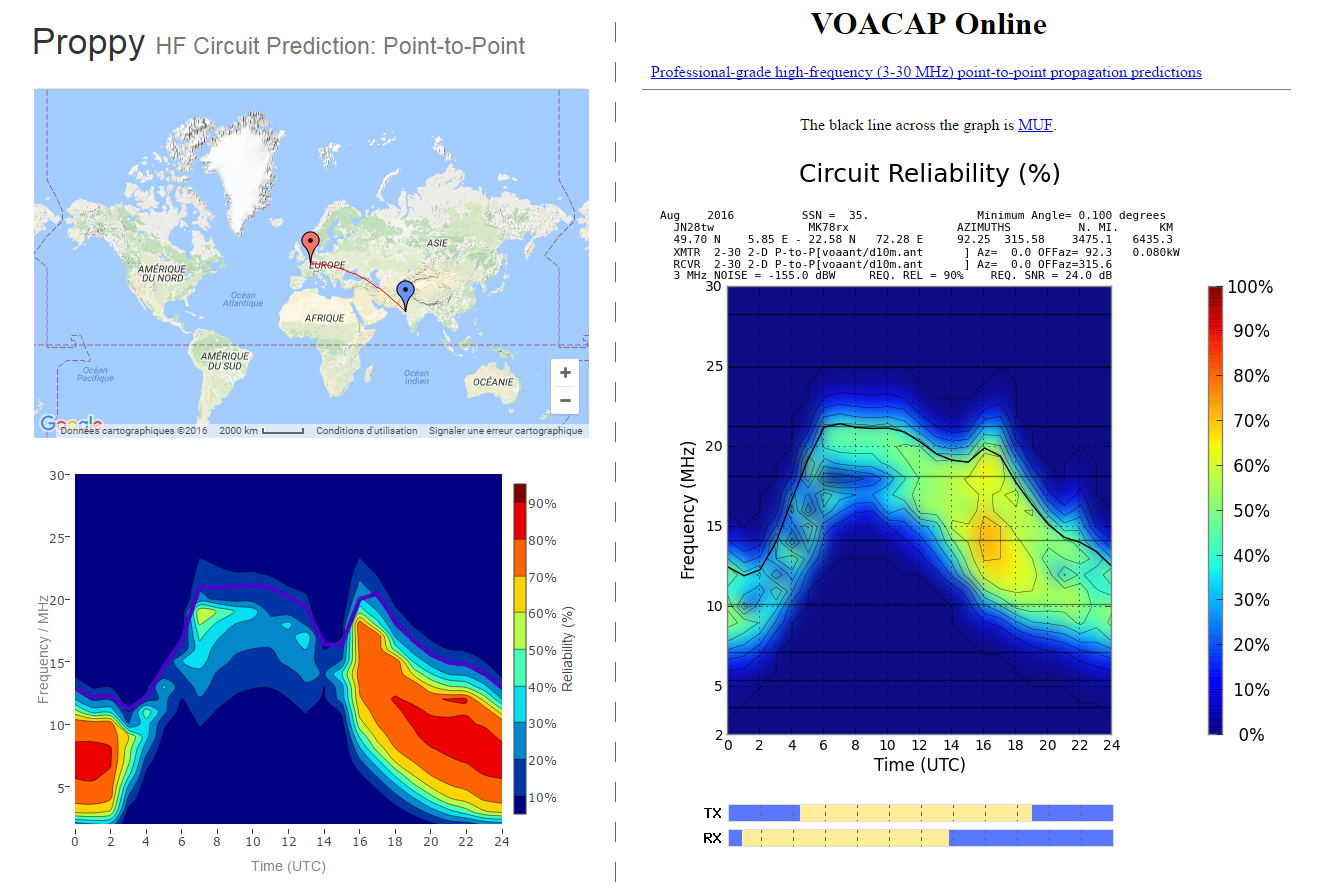
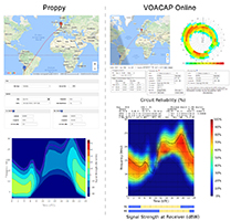
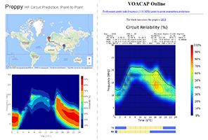
Comparisons
between two point-to-point predictions
calculated by Proppy (left part) and VOACAP Online (right part). The MUF
(as the other data) can be different because the ITURHFProp model, thresholds,
required reliability and SNR used by Proppy are not the same as in VOACAP.
Poppy is more pessimistic (e.g. Proppy uses a SNR of 13 dB for a 3 kHz bandwidth
where VOACAP uses 8 dB for a 3 kHz bandwidth), and data are derived from ITU-R F.240-7.
In addition, circuits are designed for the military use assuming the full 3 kHz bandwidth.
Future versions may extend this to 24 kHz bandwidth to support data. |
|
Note
that Proppy is able to calculate path
lengths up to 7000 km, and beyond 9000 km using an empirical formulation
based on the range defined by LUF and MUF. It is assumed to be along the
great circle in E modes up to 4000 km and via F2 modes for all distances
and specially the longest.
The
engine takes into account all the usual parameters : MUF, time
windows (currently limited to any month in the current and next
year), location, power, SSN (Smoothed-Sunspot Number from SIDC), the field
strength i.e. the transmitter frequency, power and antenna gain,
required S/N, amplitude, etc. The model also calculates the
equatorial scattering of HF signals.
D.
The bottom line
What
can we conclude from these observations ? Currently there is no way to adequately model global
irregular variations in the ionosphere on a time scale smaller than a
month. Unlike some shareware for which authors claim that
their software produces more accurate predictions by using daily and
hourly parameters, the authors of the engines used by VOACAP and Proppy
have realized that random values
cannot be predicted but can be described statistically. It is why
their engine produces monthly medians, deciles, standard deviations,
probabilities of service, etc. Such statistics are predictable and
accurate (remember the accuracy of insurance statistics), predictions
for a particular date and hour are just speculations.
Remember
also that VOACAP was initially designed for experimenting with
prediction algorithms, but the experimentation was never finished due to
lack of funding. Just take a look at the list of available prediction
methods available in VOACAP - there are 30 - and all output parameters
to understand all the extent of the problem. For example, you can specify
the month and day of prediction, but this will automatically force the
program to use URSI coefficients - which should never be done because,
according to the VOACAP authors, these coefficients produce incorrect
predictions. (Now you know why Ham CAP does not use the day of the month
either !). But as we will see in reviewing VOACAP,
there are tens of ways to produce invalid VOACAP predictions by setting
incorrect parameters. Many of them were explained in the VOACAP mailing list at
QTH.net. If you are not subscribed yet, I highly recommend you this list.
Next chapter
Requisit
and specification of amateur programs |