|
What
can we expect from a HF propagation model ?
Forecasts
reliability (VI)
In HF, reliability represents
the average monthly time availability for each hourly computation. This is a
statistical factor. Usually amateurs use a value of 50% reliability, even less
in CW. 50% means that the mean monthly level for the specified circuit would be
available during at least 15 days per month. Of course the higher the best.
This factor adding a limitation
in the computation, the higher the reliability the more conservative,
pessimistic is the estimation. Commercial circuits like the ones of VoA, BBC or RFI for example use
a 90% reliability in order that all listeners receive their signals in excellent
conditions. It means that the circuit would be available as predicted at least during 27 days per month. In a
world coverage map, the more conservative coverage area is thus also smaller.
As with any statistics, data
interpretation is the harder part of the simulation. Amateurs don't like to set
a too high reliability because the estimation is too pessimistic; we all know that
even when a simulation states that bands are closed from 15 to 10m, we have still to
interpret properly this estimation. Concerning DX contacts, does it mean that
stations located 2000 km away are also concerned by this "blackout" or
only those located over 5000 km away ?
 |
 |
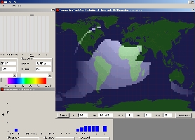
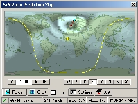
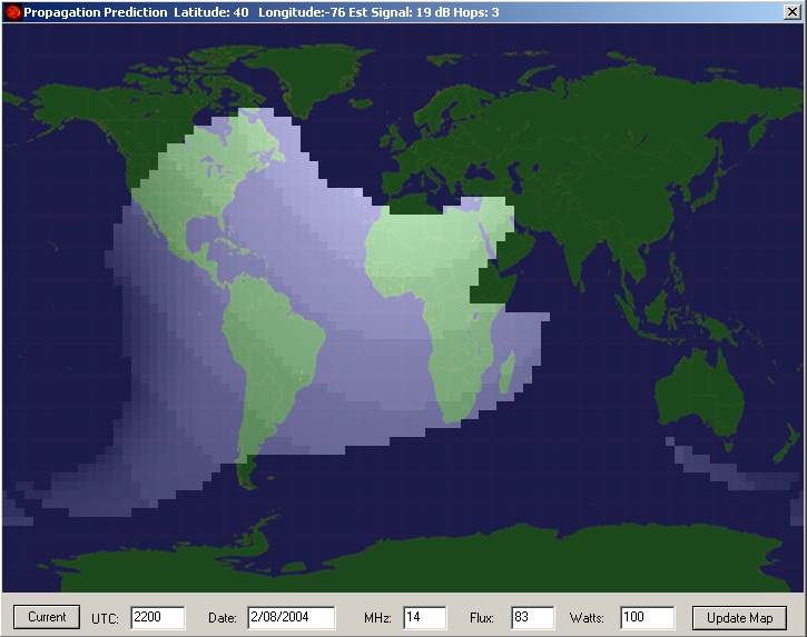
At
left a forecast calculated by DX Toolbox
for a 100 W PEP transmission from ON in
summertime by 2200 UTC on 20 meters. The audio reports
doesn't correctly match the prediction : signals from
K are readable even if they are weak (they will be
much stronger 1 to 2 hour later), FY is as strong as
expected but worst, stations from LA or UT are
predicted unreadable although they are strong, and VK8
stations (at Darwin, North of VK) using the short path, so-called unreadable,
show a strong audio. DX ToolBox displays the signal
strength but not the S/N required reliability, the power at receive station,
etc, because the program makes rough assumptions and uses always the
highest reliability. At right the point-to-point
prediction established by VOACAP for the circuit
Brussels (ON) to Darwin (VK8) at the same time.
The SNR of 50 dB shows indeed that the 20-m band in open to VK
near 2200 UTC with a S/N of 10 dB only, very weak.
Approximatively the same SNR chart but weaker (SNR of
5 dB) was predicted between ON and FY. In
the field the S-meter was strong for FY (S-6) and very
weak for VK (S-1) but with a strong audio (equivalent to
S-7 to S-9) in both cases. Both applications forecasted
well some openings but not all, and both are wrong
about some details (Signal strength to LA and UT for the
first, and SNR to FY for the second model although its
prediction for VK was correct). Of course
one sample does not represent the overall performance
of these programs. |
|
In
fact the simulation doesn't work like this. Only the propagation chart
calculated for a band, a given date and time at the required reliability give you a global estimation of
the propagation conditions at the earth scale. When you ask for a prediction
for a specified path (e.g. ON to LA as displayed in the below charts) only the
propagation conditions along this point-to-point circuit are taken into account, most of the
time using median or highly reliable values. But sometimes, even using statistical values, conditions in the field can be quite
different. The reason is related to the accuracy of models and the update of not
of "smoothed" values of the solar and geomagnetic data.
Analysis
of seven forecasts
Let's
take an example, or rather seven examples. I worked Bodo, in Norway
(67°N, 14°E) on August 8, 2004 at 12:00 UTC (SSN 29, SFI 86) using a G5RV
dipole tight in the E-W direction. Here is its radiation
pattern calculated with MultiProp
(settings are 100 W PEP, beam heading 0°, 20-m band, QRM "rural",
chart calculated for August 2004 with CCIR/Oslo Coefficients.
Most applications predicted that there was no
opening to expect to LA above 14 or 15 MHz as show graphs displayed below.
In retrospect, their accuracy was more than approximative. On the other
side, most programs using the VOACAP engine, sometimes
"updated" with real-time ionosonde data say all
the contrary, and that was indeed confirmed in the field...
Here
are forecasts calculated by seven applications recently published using,
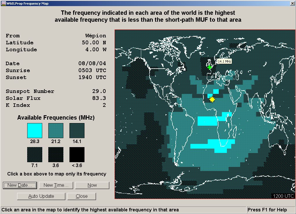
as far as possible, the same input parameters. Honor to the elder, W6ELPro
which chart is displayed at right, predicts a MUF at 14.1 MHz in Norway.
In
other charts (signal level prediction) W6ELPro predicts a field strenght in LA
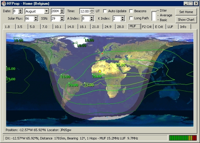
of 44 dB over 0.5 μV, thus S9+10. According to G4ILO's HFProp
(below left), DX openings are not numerous at that time and
mainly located to northern latitudes. The MUF is at 15.1 MHz at
12:00 UTC and the signal to LA is strong (meter below right in the green).
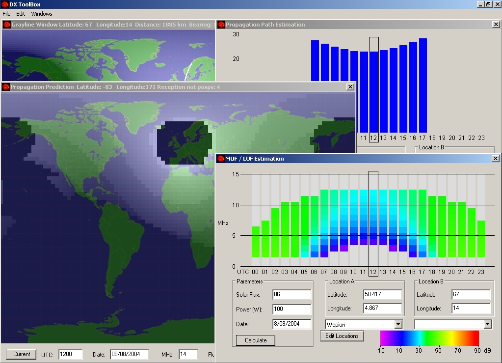
However, it does not permit to get more information. For DX
ToolBox (below center), the target location is in the silent
zone with a MUF near 13 MHz and the signal estimated to 30 dB
(cyan). Note that outside the skip
distance, the field strengh reach about 25 dB. However
its silent zone it at least 30% too wide.
Now
let's see what predict the applications using the VOACAP engine.
For WinCAP Wizard 3 (below right)
using an SNRxx of 50%, thus not too optimistic and not too pessimistic either, the SNR is over 50 dB at 12
UTC and qualified as "fair" (good) in SSB, in spite of a
strong field strength estimated at S7.5. The MUF is predicted at 13.7 MHz. This
is the first application to provide a posteriori a valuable estimation.
For
GeoAlert-Extreme Wizard
(below left) the MUF ≤ 20 m or 14 MHz over Scandinavia. According to DXAtlas
(below center), that uses real-time ionosonde data, the MUF is at 17.300 MHz over
Bodo (mid of Norway). At last, for its companion, Ham
CAP (below right) the SNR in LA is 42 dB, strong too.
Checking
these predictions with real QSOs, I noticed that contacts were possible with all european countries from EA to LA with signals up to
S-9, even on 28.5 MHz. On 20 m my reports from LA were indeed S9+, some S-units
better than predicted.
|
|
|
|
|
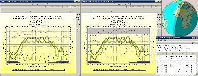
From
left to right, screen dumps from GeoAlert-Extreme
Wizard, DXAtlas (with
Ham CAP et IonoProbe), and Ham
CAP (stand-alone) for a short circuit of 2000 km between Belgium and Norway, on August 8,
2004 at 12:00 UTC.
|
|
Generally speaking we can say that upper bands were close for DXing. But not
entirely. Circuits to Spain or Norway for example shown a good S/N ratio over 50 dB.
But predictions estimated the BUF limited to 10
MHz at noon and the MUF oscillating between 13 and... 17 MHz.
If
I had to trust these predictions, theoretically I might work those countries up to 30, maybe 20m,
but not higher. However, in the field there was some activity on 17, 15 and still more on
the 10-m band where they were amateurs from EA and LA. Of
course the 10-m band was not crowded and only a handful
amateurs were on the air. And for DX stations upper bands were
indeed closed excepting a good opening to South Africa and Madagascar forecasted
by some applications.
Reliability must thus be used with care,
and preferably in addition to other estimations of the ionospheric status and
field strength (MUF, BUF, SNR, SNRxx, dBW, dB>mV, etc).
This
analysis is thus a perfect example of the art to
not always trust in charts or, if you like, to interpret them
correctly when they use statistical data instead of real-time data...
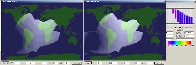
Effects
of power gain
As we told previously, amateur transmitters show an output power in a ±10 to 20 dB range (10-100-1000 W PEP).
A good propagation program should be able to show the effect of power gain on
the area coverage, and hopefully most recent programs take it into account. Chart
and maps show those
sensitivities over a ±10 dB range by using either a false-color pattern that
highlights the increasing in coverage or simply put in light a larger area on the
worldmap as shown below.
Like on the air, the increasing (or decreasing) in
signal strength is more perceptible on the weakest signals. The WinCAP
simulation shown below displays very well this effect, increasing the weakest
signals (early morning and late in the evening) of 1.5 S-unit or 10 dBW.
Such simulations can thus also be used to
show the effect of potential changes in the station's hardware (transmission
line of lower loss, receiver of higher sensitivity, use of a linear amplifier,
antenna of higher gain, etc, as many parameters took into account by VOACAP).
 |
|
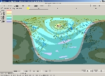
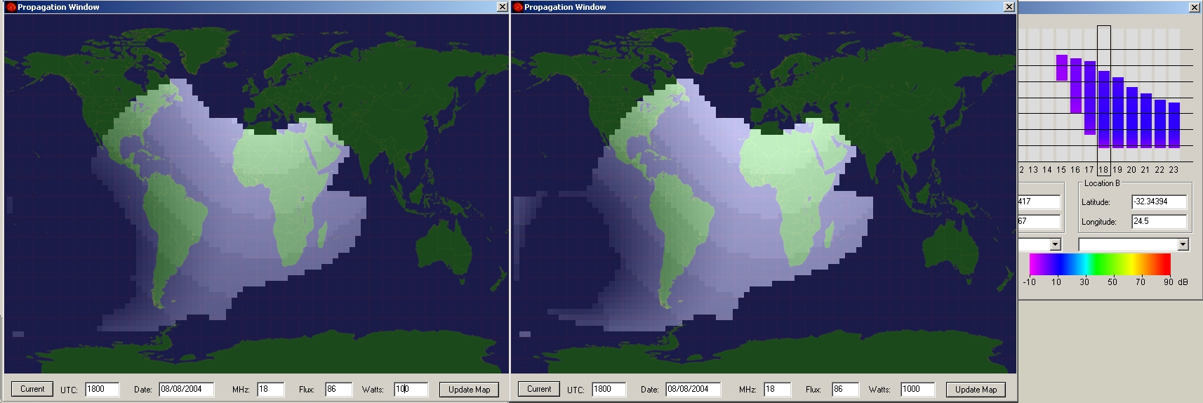
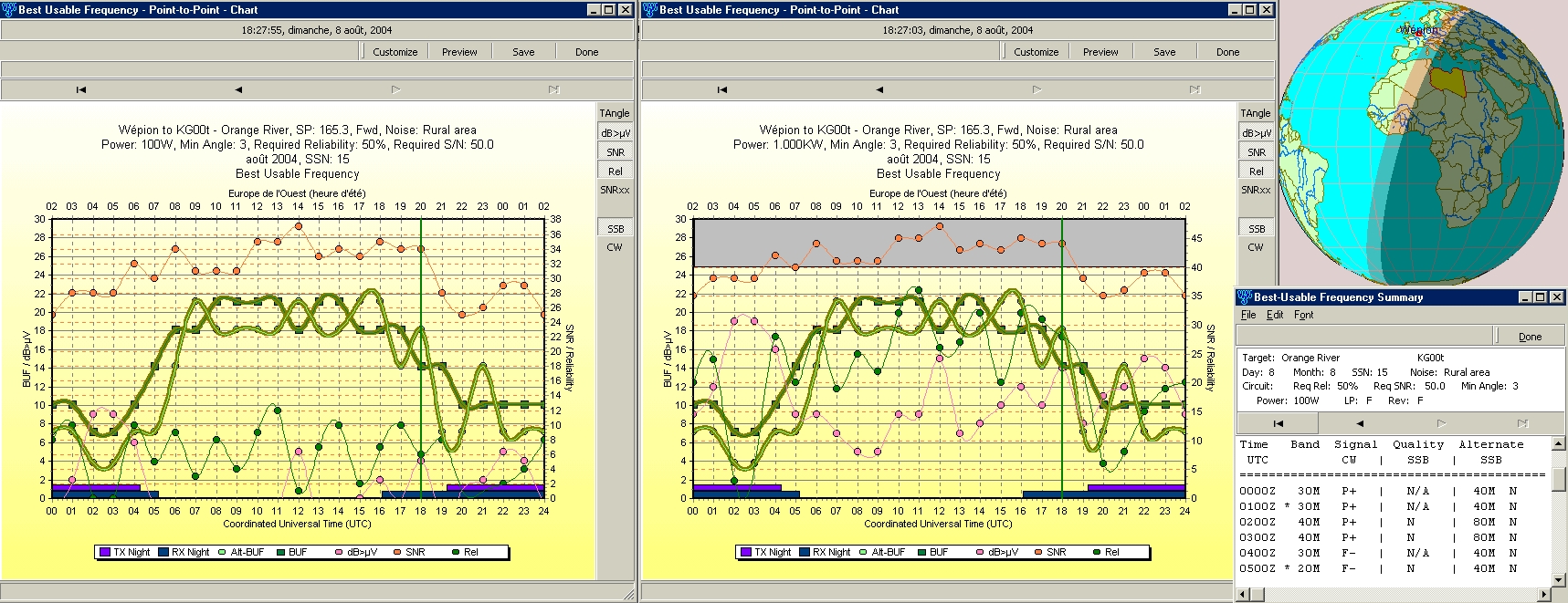
The
effect of a power gain of 10 dB (100 W to 1 kW) on
the propagation. The MUF/LUF is given for a path from ON to ZS. Above
the results displayed in DX ToolBox, below in WinCAP Wizard 3. In the best conditions, the VOACAP model
shows that the power gain does not increases the S/N ratio of
strong signals (S/N > 10 dB or > 8 dBW) but well the weakest
that jump from 8 to 18 dBW or 1.5 S-unit (S-5 to S-6.5). A higher
solar flux (e.g. SFI of 200 instead of 86 in this case) does not
change this effect. |
 |
|
Are
circuits reciprocal ?
Is the communication circuit
between New York and London "electrically" speaking identical to the
circuit from London to New York ? At first sight it is, except that we can
already note that, at daytime, the position of the sun affects the receive
station of a strong QRN. Relevant observation.
For decades, engineers and
physicists considered that the ionospheric signal propagation was essentially
the same in both directions along a given path. Excluding
short-term changes in the ionosphere (warm up, sporadic plasma clouds,
storm, aurora, etc), this is true within a few
decibels for the upper bands and in a lesser extend for the low bands as well.
However, when we take into
account SNR predictions, thus the signal quality, circuits are no more reciprocal.
These variations are primarily due to different atmospheric noise levels
at the receive site.
 |
 |
|
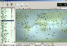
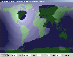
Propagation
charts calculated by DX
ToolBox for the 20-m band on August 2, 2004 22:00 UTC for paths
from respectively New York to London (left) and the opposite (right). In both
cases of course the number of hops is 3 as listed in the blue
upper bar. Both propagation estimation maps are different because at that
time the position of the Sun is simply not the same over both
QTH. In theory they are also different because the S/N
ratio at both terminals is affected by noise generated not
only by the sun but also along the path by thunderstorms,
aurora, and sometimes QRM emitted by large industrial cities.
The S/I ratio can help to predict these effects. At last, both circuits
have also different losses. However all these variables,
excepting the sun position, are not taken into account by this
application that gives only a rought estimation of the
ionosphere status, at earth scale (intensity of field
strength, MUF, etc).
|
|
In
the late '90s ACE-HF, an U.S. company managed
by Richard P.Buckner, was commissionned by the U.S.
Navy to study propagation circuits within the Atlantic area.Dick
is also author of a propagation program of the same
name using the VOACAP engine. His conclusions showed
a directional difference of as much as 12 dB in received
S/N ratios, what represents a power ratio that exceeds a
2-factor ! The source of this reciprocity failure was determined
to be the different atmospheric noise levels at either end of the
circuits. It appeared that lightning flashes from thunderstorms
that concentrated in the summertime in the Caribbean area generated an
increasing of atmospheric noise levels, similar to what we experiment on the low
bands from 40 m and up when a frontal system moves close to our receiver.
 |
|
Reciprocity
SNR differences along the circuit Nortfold, VA to Iceland and the
opposite can be as much as 12 dB and are due primarily to
different atmospheric noise levels at the receive sites. Document
created with ACE-HF. |
|
However,
if the problem is well-known, very few propagation programs
take all these effects into account. A model like VOACAP or ICEPAC for example is
ionospheric-effects oriented, this is a point-to-point signal model that only incorporates the
SSN, the date, time and the circuit properties (working conditions at both ends
of the circuit, including the ground properties and QRM at target location).
The atmospheric conditions are simply bypassed.
IRI on the contrary
or down-sized versions like DXAID or DXAtlas, tries to incorporate various processes like the electron temperature, the
auroral precipitation or the conductivity but it doesnt' take into account the
atmospheric conditions yet; maybe for after tomorrow, when a future release
of IRI-200x will be interfaced with the best weather model from the World
Meteorological Organization. That day maybe, we could say that we master almost
the atmosphere. Remain to master the geomagnetic dynamo, the sun and the space
weather models and to link all that stuff in our super meta big "sun-earth
plasma model"... A fine project without any doubt !
 |
 |
|
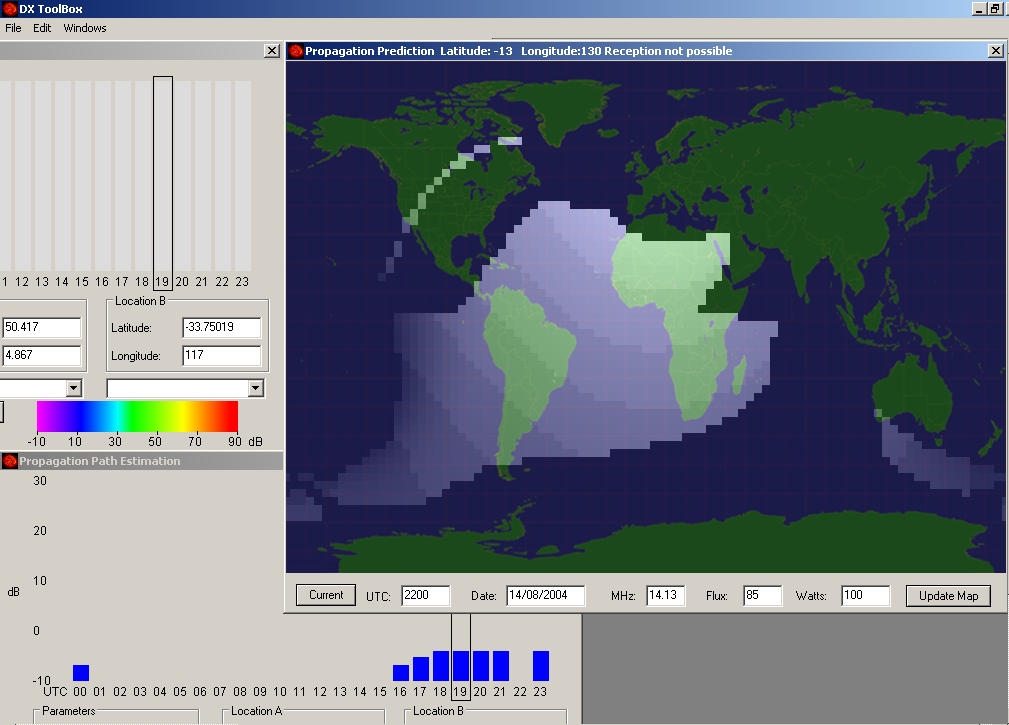
Example
of reciprocity predicted with ICEPAC for a circuit
between Belgium and Australia on August 14, 2004 (SSN
85). The SNR is set to 50 dB, SNR required reliability
SNRxx to 50% for a power of 100 W PEP in both
antennas. Simulations are respectively viewed from the
receive location in VK (left using a 3-element Yagi
and from the receive location in ON using a 31m long
dipole (right). Variations do not exceed 5 dBW or half
a S-unit. At the time of the QSO (22 UTC, local
midnight in ON, 7 am in VK) the position of the sun
and thus the ionization level of the F-layer was very
different over each location. Thanks to accurate
algorithms, ICEPAC predicted that signal power
at both receive locations 'd be identical
(-146.44 dBW or S2) and the SNR over +16 dB, thus very
weak. On the air VK signal arrived indeed very weak (S-1) but with a
strong audio (equivalent to S-7 or S-9). |
|
Now
that you master or almost the main parameters used in the VOACAP model,
I suggest you to read my review of VOACAP
to understand how powerful and more flexible it is compared to simpler
prediction programs.
For
more information
On
this site:
Review
of HF propagation analysis and prediction programs
VOACAP
propagation program review
DX
ToolBox propagation program review
WinCAP
Wizard 3 propagation program review
HFProp
propagation program review
Online
VOACAP predictions
VOACAP
online
VOACAP
module of DX Summit cluster (clic on a call sign to get predictions)
Proppy
Activities
on bands via DX Heat (clic on a call sign and select the headset to listen
to the QSO)
Propagation
tutorials:
AC6LA's
MultiProp tutorial (program interfacing VOACAP and MultiNEC
models)
HF
Radio Propagation Primer, by AE4RV (Tutorial, Flash presentation)
Radio
wave propagation (chapter 2), TPUB Tutorial
International
Journal of Geomagnetism and Aeronomy (AGU, many studies related to geomagnetic
effects)
Analytical
Calculation of the Radio Wave Trajectory in the Ionosphere, J.Młynarczyk et al.
Propagation
books:
Physics
of the Upper Polar Atmosphere, by A. Brekke, John Wiley & Sons Inc, 1997
The
Little Pistol's Guide to HF Propagation, by Robert R. Brown, Worldradio
Books, 1996
The
New Shortwave Propagation Handbook, by Jacobs, Cohen and Rose, CQ
Communications, Inc., 1995
Radio
Amateurs Guide to the Ionosphere, by Leo F. McNamara, Krieger
Publ.Corp.,1994
Ionospheric
Radio (IEE Electromagnetic Waves Series, Vol. 31) by K.Davies, Inspec/Iee,
1990
Radio
Wave Propagation (HF Bands): Radio Amateur's Guide, by F.Judd,
Butterworth-Heinemann, 1987
Propagation
Studies, RSGB
ARRL's
Bookshop
RSGB's
shop
Ionospheric
models:
PropLab
Pro (software)
AIAA
Guide to Reference and Standard Ionosphere Models (G-034-1998)
CODE
GIM model
The
IRI On-Line Model
International
Reference Ionosphere (IRI-2001)
STORM model
Substorm
models
Signal
Propagation (VOACAP, Jones-Stephenson, RIBG and EICM models)
Real-Time
UAF Eulerian Polar Ionosphere Model (UAF-EPPIM)
Global
Ionosphere Maps Produced by CODE
ESOC
Ionosphere Monitoring Facility (IONMON)
WBMOD
Ionospheric Scintillation Model
Thermosphere
Ionosphere General Circulation Model (TIGCM)
Sheffield
University Plasmasphere-Ionosphere model (SUPIM)
Coupled
Thermosphere Ionosphere Plasmasphere Model (CTIP)
Coupled
Thermosphere Ionosphere Model (CTIM/CTIP/CMAT)
Sheffield
Coupled Thermosphere-Ionosphere-Plasmasphere model (SCTIP)
Coupled
Ionospheric-Thermosphere-Electrodyanmics Forecast Model (CItEFM)
Mid-latitude
Ionosphere Model (MIM)
Multi-Quasi-Parabolic
model (MQP)
Low-Latitude
Ionosphere Sector model (LLIONS)
Cellular
model of the magnetosphere-ionosphere substorm activity (PDF), PGI, Russia
Mass-Spectrometer-Incoherent-Scatter
(NRLMSISE-00)
Marshall
Engineering Thermosphere (MET-V 2.0)
Drag
Temperature Model (DTMB78)
Horizontal
Wind Model (HWM93)
etc.
Back to Menu |


