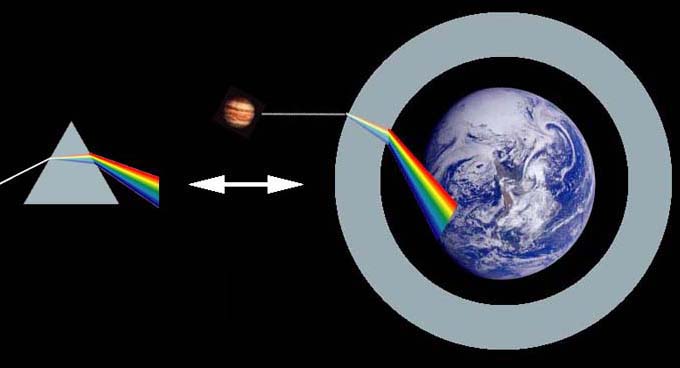
The atmospheric dispersion is an aberration introduced by the Earth's atmosphere generating a vertical deflection of light coming from any celestial body. This deviation is different as function of the wavelength: indeed, blue radiation is deflected more than red one, generating red stripe on one side of the observed object and blue on the other one. For CCD imaging, the resolution is also more or less strongly degraded and this despite the use of band-pass color filters.
The Atmospheric Dispersion Corrector (ADC) is an optical device based on a tunable prisms assembly aiming at compensating this deflection.
The atmospheric dispersion phenomenon
Before reaching the telescope, the light coming from extra-terrestrial objects must first cross the Earth atmosphere. That's the point where the refraction phenomenon is going to act on this light in deviating it, generating an effect similar to the "broken" stick plunged into the water. The phenomenon of refraction is due to the change of the light propagation environment, from the vacuum space to the Earth atmosphere. Every medium is characterized by its propagation index n
It would not be a problem for CCD work if this deviation was homogeneous in frequency: but unfortunately, it is not the case! Indeed, the blue radiance is the most deviated and the red is the least: the atmosphere thus behaves as a large-scale prism.
This phenomenon is the atmospheric dispersion due to the fact that Earth atmosphere index is function of the light frequency.
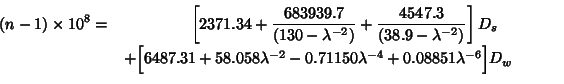
Many studies have been made, aiming at building a model of Earth atmosphere index. J.C Owens' one seems to be the most widely used as seen in astronomic literature, study which led to the following equations:
where:
• Ds is the density factor associated to a dry air and is given by the following formula:
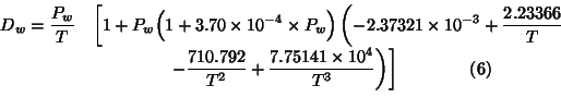
• Dw is the density factor associated to the water vapour and is given by the following formula:
with also the following hypotheses:
• Ps is the dry air partial pressure. The value of Ps is linked to the altitude h (in meters) through the following expression:
Ps = P0 *exp(- h / 7000), with P0 = 1013,25 mb
• Pw is the water vapour partial pressure. This pressure is linked to the temperature t (in Celsius) and the Hygrometry level (in %) through the following expression:
The units used in the formulas above are: pression in millibars, wavelength in microns and temperature in Kelvin.
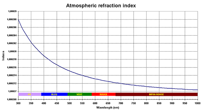
Based on this theory, it can thus be possible to draw the atmospheric index as a function of light wavelength:
assuming following atmospheric parameters:
• t = 15°C
• h = 150 m
• Hygrometry = 50%
It can be noticed a stronger variability in the blue than in the red (the slope of variation of the index is higher for short wavelength). The blue layer will thus suffer the most of this phenomenon. For us astronomers, it introduces in the eyepiece or with a CCD, a shift of color layers visible as a red border on one side of the planet and a blue one on the other side.
This phenomenon is important all the more as the angle between the direction of incoming light and the normal to the Earth atmosphere is large thus for objects observed or imaged at low elevation.
This problem can be partly solved with imagery by re-aligning the red, green and blue layers: either during the RGB registration proces for a black and white CCD used with color filters, or for a color image by dividing it into its red, green and blue components and the same re-alignment process.
This correction is only partially corrected through this process. The atmospheric dispersion inside each filter pass-band is not compensated: and this dispersion can be large, particularly for the blue layer. This intra-band effect will generate bad quality images, similar to a generalised blurring. Moreover, for a luminance imaging as used in LRGB technics, the correction is not possible. The dispersion greatly reduces then the capacities of the B&W CCD. To prove this assertion, here is a simulation of dispersion effect as a function of the elevation, using the theory exposed before:
The curve above has been computed using Astronomik RGB filters and SKYnyx 2.0M sensor characteristics.
Take the example of a 200mm telescope. The theoretical resolution of this telescope can be computed with a criterion a little lower than that of Rayleigh and Dawes, and adapted to the experimental results obtained with planetary dedicated telescopes (cf page 7 of the book " Observing and Photographing the Solar System " by Dobbins, Parker and Capen): resolution = 4,41 / diameter (inches) ie approximately 0,53 for a 200 mm.
It can be noted that for such a telescope, the elevation under which the atmospheric dispersion begins to degrade the scope resolution (as determined with the formula above) is of 58° for the blue layer, 35° for the green and 25° for the red.
One could however object me that in most of the cases, the turbulence will prevent the use of a scope to its ultimate resolution capacity, a problem much more important and limitating than this atmospheric dispersion phenomenon. May be, but for the nights with a great seeing which are so rare and thus to be fully exploited, the dispersion might become the main contributor whereas there are solutions to compensate it (see below). Moreover, for the Luminance layer (for LRGB technics) the dispersion reaches levels similar to the turbulence ones for fairly high elevations: 1 arcsec of dispersion is obtained for 53° of elevation ! The correction of the dispersion allows thus to use the LRGB technics at its full capacity almost every great nights.
Application to planetary observation and imaging
On the previous graph, I have indicated the present maximal elevation of Jupiter (25° in 2007) in North hemisphere. The dispersion is just acceptable for the red layer, reach around 0.8 arcsec for the green and is particularly destructive for the blue with 1.4 arcsec. For the Luminance, it's even worse ....
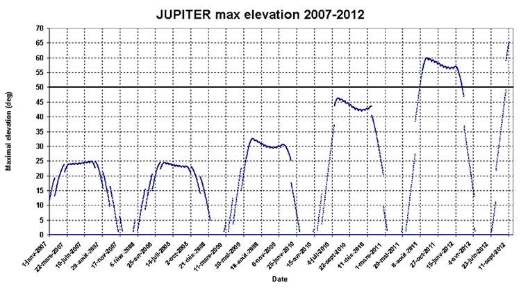
Unfortunately, for Jupiter, these bad visibility conditions in North hemisphere will remain for a while. The graph hereafter provides the maximal elevations until 2012 with following hypothesis:
• night defined by an elevation of Sun below -10°,
• an observation latitude being Nice one.
It can thus be seen that Jupiter won't exceed an elevation of 50° until half of 2011, giving 4 Jupiter apparitions with bad dispersion conditions.
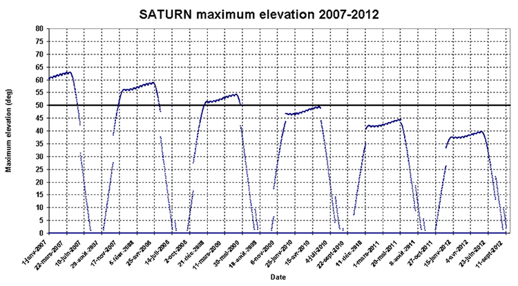
For Saturn, the situation will get worse for the next apparitions as it can be seen in the graph hereafter (made with the same hypothesis as above):
The 2008 and 2009 apparitions will be above the 50° elevation criteria (in 2009, the slots in such conditions will be very short). After 2010, the conditions will become degraded.
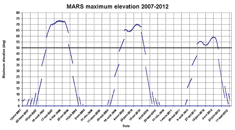
At last, for Mars, the following graph can be drawn:
The situation remain acceptable until 2012 and will become unfavourable for the 2014 apparition.
The ADC = Atmospheric Dispersion Corrector
The studies made since many years about the atmospheric dispersion phenomenon and the ways to compensate it, has shown that the induced chromatic shift can be corrected at 1st order by the use of glass prisms. Unfortunately, no glass has a refraction index profile similar to the Earth atmosphere one, over a large bandwidth. Some combinations can however bring a satisfying correction over a reduced bandwidth (typically 350-900 nm), which is largely enough for amateur uses: our CCD sensors have in any case a low if not no sensibility out of this range.
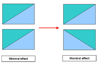
2 types of prisms combinations are commonly used:
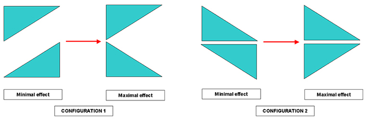
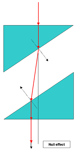
• 1 pair of simple prisms which can be rotated in reverse ways and made of the same glass: that's the so-called Risley prisms. The 1st prism deviates the light and the second one brings it back partially depending on the angle between both prisms. 2 prisms layouts are possible (configuration 1 and 2 on the graph below):
The advantage of such a solution is its great simplicity: 2 prisms only have to be manufactured and the rotation system is simple to build.
However, this system has the drawback to introduce a lateral deviation of incoming light, even in null position. During the prisms tunig, this characteristics induces for instance an important motion of the object to be pictured or observed. During the corrector tuning, the object has thus to be re-centered systematically.
• An other solution is made of 1 pair of Amici prisms. This configuration is similar to the previous one, but instead of having simple prisms, this system uses 2 prisms made of glasses with different refraction index.
This solution allows to avoid the lateral deviation mentioned for the 1st design. But the multiple glass elements introduced in the optical path imply a lower light transmission particularly in UV domain for which most of glasses have poor transparency.
For the correctors used in great Observatories (La Silla, Kitty Peak, ...) the lack of lateral deviation is of a great importance due to the very precise measurements made in these installations: the configuration #2 with Amici prisms is thus preferred.
For correctors proposed for amateur astronomers, Risley prisms are preferred in order to keep the system simple to manufacture, to use and with costs low enough.
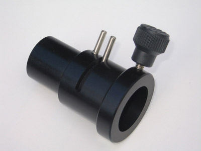
2 models are presently proposed, with 31.75 mm (1''1/4) interface:
• the ASTROVID corrector (not sold anymore) is made of a simple prism with deviation angle of 2° or 4° (1). To get a tunable Risley system, 2 correctors must thus be bought and installed one over the other. The tubes have then to be turned differentially to get a variable dispersion correction.
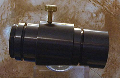
• The Astro Systems Holland (ASH) corrector which is made of 2 prisms with deviation angle of 4° (1), installed in the same fairing with 2 levers allowing the differential rotation.
The ASH corrector is obviously more compact and much more easy to use: this is the system I bought. The levers allow to tune the corrector whitout turning a whole mechanical part including the CCD camera as it is the case with the Astrovid corrector. The tuning precision is also much better.
It has to be noted that the ASH prism are declared to be surfaced at lambda/4 to be compared to the lambda/10 announced by Astrovid. But in practice, this difference induces no dramatic degradations.
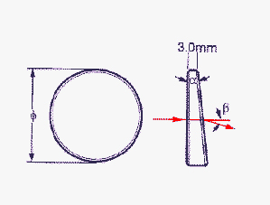
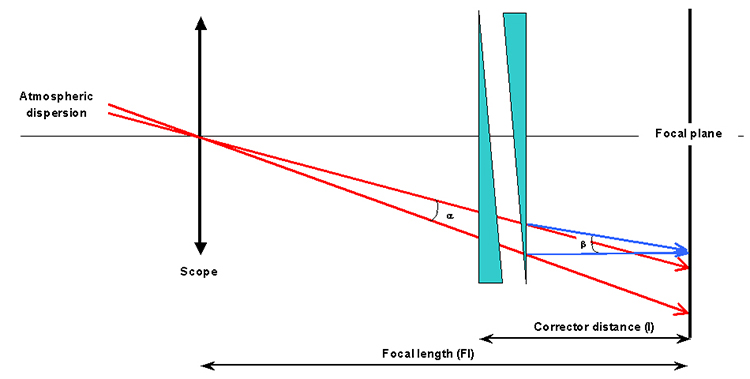
(1) a precision about deviation angle should be made. This angle is often mentioned in articles dedicated to dispersion correctors. There is an ambiguity with another angle:
• either the wedge angle (alpha angle on the scheme under),
• or the prism deviation angle (angle beta)
The link between both angles is function of the glass refraction index and of light wavelength. In general, when no precision is made, the angle mentioned corresponds to the deviation angle beta.
ASH corrector analysis
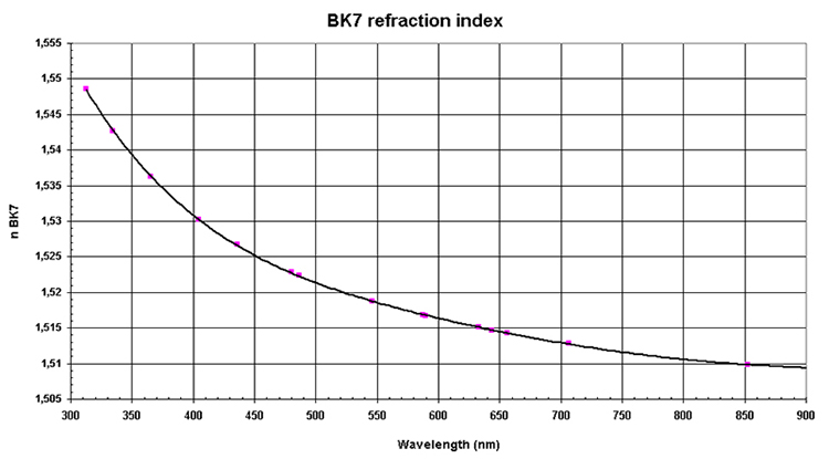
The ASH corrector prisms are made of BK7. The refraction index of this glass is provided on the graph hereafter as function of the wavelength:
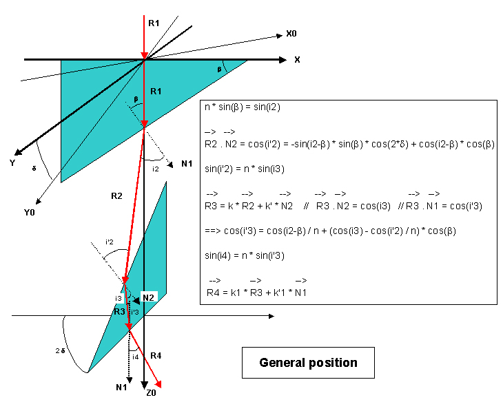
The Risley prisms of the ASH corrector are assembled in the configuration 1 described before. The configuration of the corrector is figured on the following scheme in an any configuration with associated Snell-Descartes formulas:
On this scheme, the trihedral X0Y0Z0 is fixed and linked to the corrector body whereas the trihedral XYZo is linked to the first prism and thus is turning with it with an angle Delta relative to the XoYoZo trihedral. The second prism turns in a reverse way of an angle -Delta, implying that both prisms are separated by an angle of 2 * Delta.
The computation of R4 output vector shows also an interresting property of the corrector: whatever the Delta angle and the index n, R4 is always in the plane (YoZo) meaning that its component along Xo is null. By orientating the corrector so that Xo is horizontal, the vertical dispersion generated by Earth atmosphere can be corrected by acting on the levers symetrically without having to turn the main body.
The formulas provide the deviation i4 generated by the prisms for a given wavelength. By doing this computation for 2 wavelengths, the dispersion generated by the corrector can be obtained.
This dispersion shall compensate the atmosphere one. The efficiency of the corrector is function of its positionning relative to the focal plane as well as the focal length of the system. The following scheme provides this link:
It can be noted that for a given atmospheric dispersion, the more the corrector will be near the focal plane, the higher the correction will have to be large ie the higher the required angle i4 the higher the angle between both prisms.
The relation between atmospheric and corrector dispersion is the following one:
Disp corrector = Disp atmospheric * (Fl - l) / l
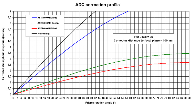
The scheme below synthetizes all these computations by giving the correction generated by the ASH ADC function of the prisms rotation:
These curves are based on the following hypothesis:
• RGB Astronomik filters bandwidth,
• a focal length of 7600 mm (F/D of 35 for a 200 mm scope) ,
• a distance between the corrector and the focal plane of 100 mm, which corresponds to my classical setup.
The correction curve on the Luminance is also provided. It has been computed for a wider bandwidth than previously mentioned ie 450-760 nm. This bandwidth corresponds to the W47 filter one, this filter being transparent also to Infra-red light.
Why the W47 filter ? Because of this IR leakage which will allow to calibrate the corrector. Indeed, with a CCD camera equiped with such a filter, by targeting a star at a given elevation, 2 spots can be detected: the first one corresponds to the star as seen in violet wavelength, and the second one to the same star in Infra-red. These 2 spots are not merged because of the atmospheric dispersion, their distance being proportional to this dispersion and thus to the targeted star elevation.
The corrector is then installed in the optical path. By turning symetrically the levers, the 2 spots come closer until they merge : at this point, the tuning and dispersion correction are optimal.
In fact, the correction is optmized only for Violet and IR wavelengths: inside this interval, the BK7 index curve being not perfectly identical to atmosphere one, the correction is not total. I have plotted for different elevations, the residual errors of the corrector calibrated with this method:
Here too, I have taken the same hypothesis for filters bandwidth, for corrector distance from the focal plane and for the systemfocal length.
An excellent correction of the atmospheric dispersion can be noticed. Giving an arbitrary criterion of correction error lower than half the theoretical telescope resolution, it can be considered that the correction is efficient for elevation higher than 10°. In practice, under an elevation of 15°, the local or atmospheric turbulence will always prevent to reach the ultimate limits of the system.
For the particular case of Jupiter, with an elevation of 25°, the dispersion correction error is of 0.1 arcsec for the blue layer, 0.05 arcsec for the green and the red. These values should be compared to the 1.4 arcsec of the atmospheric dispersion without the corrector in the blue channel : the ADC has thus corrected more than 90% of the dispersion !
ASH corrector use
After a good period of use of ASH corrector, few use guidelines can be emitted:
• the corrector shall be used only with F/D ratio high enough, above 10. It must so be positionned after the Barlow on the optical path. If not, the corrector may introduce a noticeable astigmatism,
• the corrector levers in null position, shall be placed horizontally one the target object is acquired. It allows the corrector to work in the vertical plane ie in the same way Earth atmosphere does. 2 positions are possible, but only one is acting in the proper way, the other one amplifying the dispersion.
The Atmospheric Dispersion Corrector (ADC) is an optical device based on a tunable prisms assembly aiming at compensating this deflection.
The atmospheric dispersion phenomenon
Before reaching the telescope, the light coming from extra-terrestrial objects must first cross the Earth atmosphere. That's the point where the refraction phenomenon is going to act on this light in deviating it, generating an effect similar to the "broken" stick plunged into the water. The phenomenon of refraction is due to the change of the light propagation environment, from the vacuum space to the Earth atmosphere. Every medium is characterized by its propagation index n
It would not be a problem for CCD work if this deviation was homogeneous in frequency: but unfortunately, it is not the case! Indeed, the blue radiance is the most deviated and the red is the least: the atmosphere thus behaves as a large-scale prism.
This phenomenon is the atmospheric dispersion due to the fact that Earth atmosphere index is function of the light frequency.
Many studies have been made, aiming at building a model of Earth atmosphere index. J.C Owens' one seems to be the most widely used as seen in astronomic literature, study which led to the following equations:
where:
• Ds is the density factor associated to a dry air and is given by the following formula:
• Dw is the density factor associated to the water vapour and is given by the following formula:
with also the following hypotheses:
• Ps is the dry air partial pressure. The value of Ps is linked to the altitude h (in meters) through the following expression:
Ps = P0 *exp(- h / 7000), with P0 = 1013,25 mb
• Pw is the water vapour partial pressure. This pressure is linked to the temperature t (in Celsius) and the Hygrometry level (in %) through the following expression:
The units used in the formulas above are: pression in millibars, wavelength in microns and temperature in Kelvin.
Based on this theory, it can thus be possible to draw the atmospheric index as a function of light wavelength:
assuming following atmospheric parameters:
• t = 15°C
• h = 150 m
• Hygrometry = 50%
It can be noticed a stronger variability in the blue than in the red (the slope of variation of the index is higher for short wavelength). The blue layer will thus suffer the most of this phenomenon. For us astronomers, it introduces in the eyepiece or with a CCD, a shift of color layers visible as a red border on one side of the planet and a blue one on the other side.
This phenomenon is important all the more as the angle between the direction of incoming light and the normal to the Earth atmosphere is large thus for objects observed or imaged at low elevation.
This problem can be partly solved with imagery by re-aligning the red, green and blue layers: either during the RGB registration proces for a black and white CCD used with color filters, or for a color image by dividing it into its red, green and blue components and the same re-alignment process.
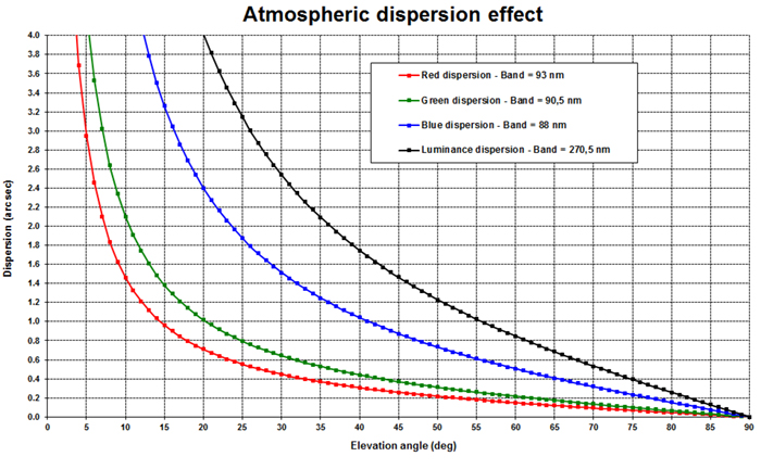
This correction is only partially corrected through this process. The atmospheric dispersion inside each filter pass-band is not compensated: and this dispersion can be large, particularly for the blue layer. This intra-band effect will generate bad quality images, similar to a generalised blurring. Moreover, for a luminance imaging as used in LRGB technics, the correction is not possible. The dispersion greatly reduces then the capacities of the B&W CCD. To prove this assertion, here is a simulation of dispersion effect as a function of the elevation, using the theory exposed before:
The curve above has been computed using Astronomik RGB filters and SKYnyx 2.0M sensor characteristics.
Take the example of a 200mm telescope. The theoretical resolution of this telescope can be computed with a criterion a little lower than that of Rayleigh and Dawes, and adapted to the experimental results obtained with planetary dedicated telescopes (cf page 7 of the book " Observing and Photographing the Solar System " by Dobbins, Parker and Capen): resolution = 4,41 / diameter (inches) ie approximately 0,53 for a 200 mm.
It can be noted that for such a telescope, the elevation under which the atmospheric dispersion begins to degrade the scope resolution (as determined with the formula above) is of 58° for the blue layer, 35° for the green and 25° for the red.
One could however object me that in most of the cases, the turbulence will prevent the use of a scope to its ultimate resolution capacity, a problem much more important and limitating than this atmospheric dispersion phenomenon. May be, but for the nights with a great seeing which are so rare and thus to be fully exploited, the dispersion might become the main contributor whereas there are solutions to compensate it (see below). Moreover, for the Luminance layer (for LRGB technics) the dispersion reaches levels similar to the turbulence ones for fairly high elevations: 1 arcsec of dispersion is obtained for 53° of elevation ! The correction of the dispersion allows thus to use the LRGB technics at its full capacity almost every great nights.
Application to planetary observation and imaging
On the previous graph, I have indicated the present maximal elevation of Jupiter (25° in 2007) in North hemisphere. The dispersion is just acceptable for the red layer, reach around 0.8 arcsec for the green and is particularly destructive for the blue with 1.4 arcsec. For the Luminance, it's even worse ....
Unfortunately, for Jupiter, these bad visibility conditions in North hemisphere will remain for a while. The graph hereafter provides the maximal elevations until 2012 with following hypothesis:
• night defined by an elevation of Sun below -10°,
• an observation latitude being Nice one.
It can thus be seen that Jupiter won't exceed an elevation of 50° until half of 2011, giving 4 Jupiter apparitions with bad dispersion conditions.
For Saturn, the situation will get worse for the next apparitions as it can be seen in the graph hereafter (made with the same hypothesis as above):
The 2008 and 2009 apparitions will be above the 50° elevation criteria (in 2009, the slots in such conditions will be very short). After 2010, the conditions will become degraded.
At last, for Mars, the following graph can be drawn:
The situation remain acceptable until 2012 and will become unfavourable for the 2014 apparition.
The ADC = Atmospheric Dispersion Corrector
The studies made since many years about the atmospheric dispersion phenomenon and the ways to compensate it, has shown that the induced chromatic shift can be corrected at 1st order by the use of glass prisms. Unfortunately, no glass has a refraction index profile similar to the Earth atmosphere one, over a large bandwidth. Some combinations can however bring a satisfying correction over a reduced bandwidth (typically 350-900 nm), which is largely enough for amateur uses: our CCD sensors have in any case a low if not no sensibility out of this range.
2 types of prisms combinations are commonly used:
• 1 pair of simple prisms which can be rotated in reverse ways and made of the same glass: that's the so-called Risley prisms. The 1st prism deviates the light and the second one brings it back partially depending on the angle between both prisms. 2 prisms layouts are possible (configuration 1 and 2 on the graph below):
The advantage of such a solution is its great simplicity: 2 prisms only have to be manufactured and the rotation system is simple to build.
However, this system has the drawback to introduce a lateral deviation of incoming light, even in null position. During the prisms tunig, this characteristics induces for instance an important motion of the object to be pictured or observed. During the corrector tuning, the object has thus to be re-centered systematically.
• An other solution is made of 1 pair of Amici prisms. This configuration is similar to the previous one, but instead of having simple prisms, this system uses 2 prisms made of glasses with different refraction index.
This solution allows to avoid the lateral deviation mentioned for the 1st design. But the multiple glass elements introduced in the optical path imply a lower light transmission particularly in UV domain for which most of glasses have poor transparency.
For the correctors used in great Observatories (La Silla, Kitty Peak, ...) the lack of lateral deviation is of a great importance due to the very precise measurements made in these installations: the configuration #2 with Amici prisms is thus preferred.
For correctors proposed for amateur astronomers, Risley prisms are preferred in order to keep the system simple to manufacture, to use and with costs low enough.
2 models are presently proposed, with 31.75 mm (1''1/4) interface:
• the ASTROVID corrector (not sold anymore) is made of a simple prism with deviation angle of 2° or 4° (1). To get a tunable Risley system, 2 correctors must thus be bought and installed one over the other. The tubes have then to be turned differentially to get a variable dispersion correction.
• The Astro Systems Holland (ASH) corrector which is made of 2 prisms with deviation angle of 4° (1), installed in the same fairing with 2 levers allowing the differential rotation.
The ASH corrector is obviously more compact and much more easy to use: this is the system I bought. The levers allow to tune the corrector whitout turning a whole mechanical part including the CCD camera as it is the case with the Astrovid corrector. The tuning precision is also much better.
It has to be noted that the ASH prism are declared to be surfaced at lambda/4 to be compared to the lambda/10 announced by Astrovid. But in practice, this difference induces no dramatic degradations.
(1) a precision about deviation angle should be made. This angle is often mentioned in articles dedicated to dispersion correctors. There is an ambiguity with another angle:
• either the wedge angle (alpha angle on the scheme under),
• or the prism deviation angle (angle beta)
The link between both angles is function of the glass refraction index and of light wavelength. In general, when no precision is made, the angle mentioned corresponds to the deviation angle beta.
ASH corrector analysis
The ASH corrector prisms are made of BK7. The refraction index of this glass is provided on the graph hereafter as function of the wavelength:
The Risley prisms of the ASH corrector are assembled in the configuration 1 described before. The configuration of the corrector is figured on the following scheme in an any configuration with associated Snell-Descartes formulas:
On this scheme, the trihedral X0Y0Z0 is fixed and linked to the corrector body whereas the trihedral XYZo is linked to the first prism and thus is turning with it with an angle Delta relative to the XoYoZo trihedral. The second prism turns in a reverse way of an angle -Delta, implying that both prisms are separated by an angle of 2 * Delta.
The computation of R4 output vector shows also an interresting property of the corrector: whatever the Delta angle and the index n, R4 is always in the plane (YoZo) meaning that its component along Xo is null. By orientating the corrector so that Xo is horizontal, the vertical dispersion generated by Earth atmosphere can be corrected by acting on the levers symetrically without having to turn the main body.
The formulas provide the deviation i4 generated by the prisms for a given wavelength. By doing this computation for 2 wavelengths, the dispersion generated by the corrector can be obtained.
This dispersion shall compensate the atmosphere one. The efficiency of the corrector is function of its positionning relative to the focal plane as well as the focal length of the system. The following scheme provides this link:
It can be noted that for a given atmospheric dispersion, the more the corrector will be near the focal plane, the higher the correction will have to be large ie the higher the required angle i4 the higher the angle between both prisms.
The relation between atmospheric and corrector dispersion is the following one:
Disp corrector = Disp atmospheric * (Fl - l) / l
The scheme below synthetizes all these computations by giving the correction generated by the ASH ADC function of the prisms rotation:
These curves are based on the following hypothesis:
• RGB Astronomik filters bandwidth,
• a focal length of 7600 mm (F/D of 35 for a 200 mm scope) ,
• a distance between the corrector and the focal plane of 100 mm, which corresponds to my classical setup.
The correction curve on the Luminance is also provided. It has been computed for a wider bandwidth than previously mentioned ie 450-760 nm. This bandwidth corresponds to the W47 filter one, this filter being transparent also to Infra-red light.
Why the W47 filter ? Because of this IR leakage which will allow to calibrate the corrector. Indeed, with a CCD camera equiped with such a filter, by targeting a star at a given elevation, 2 spots can be detected: the first one corresponds to the star as seen in violet wavelength, and the second one to the same star in Infra-red. These 2 spots are not merged because of the atmospheric dispersion, their distance being proportional to this dispersion and thus to the targeted star elevation.
The corrector is then installed in the optical path. By turning symetrically the levers, the 2 spots come closer until they merge : at this point, the tuning and dispersion correction are optimal.
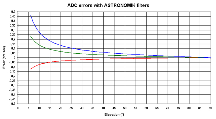
In fact, the correction is optmized only for Violet and IR wavelengths: inside this interval, the BK7 index curve being not perfectly identical to atmosphere one, the correction is not total. I have plotted for different elevations, the residual errors of the corrector calibrated with this method:
Here too, I have taken the same hypothesis for filters bandwidth, for corrector distance from the focal plane and for the systemfocal length.
An excellent correction of the atmospheric dispersion can be noticed. Giving an arbitrary criterion of correction error lower than half the theoretical telescope resolution, it can be considered that the correction is efficient for elevation higher than 10°. In practice, under an elevation of 15°, the local or atmospheric turbulence will always prevent to reach the ultimate limits of the system.
For the particular case of Jupiter, with an elevation of 25°, the dispersion correction error is of 0.1 arcsec for the blue layer, 0.05 arcsec for the green and the red. These values should be compared to the 1.4 arcsec of the atmospheric dispersion without the corrector in the blue channel : the ADC has thus corrected more than 90% of the dispersion !
ASH corrector use
After a good period of use of ASH corrector, few use guidelines can be emitted:
• the corrector shall be used only with F/D ratio high enough, above 10. It must so be positionned after the Barlow on the optical path. If not, the corrector may introduce a noticeable astigmatism,
• the corrector levers in null position, shall be placed horizontally one the target object is acquired. It allows the corrector to work in the vertical plane ie in the same way Earth atmosphere does. 2 positions are possible, but only one is acting in the proper way, the other one amplifying the dispersion.
Atmospheric dispersion
Astrophotographie Planétaire
by Jean-Pierre Prost

Pages en Français


Copyright © 2009 by Jean-Pierre Prost · All Rights reserved · E-Mail: astrojp (at) free.fr

Vous avez un commentaire ?
Any comment ?
Any comment ?
signez mon livre d'or