| Tutorial- lesson 11 - Full processing session |
Tutorial- lesson 11 - Full processing session
![]()
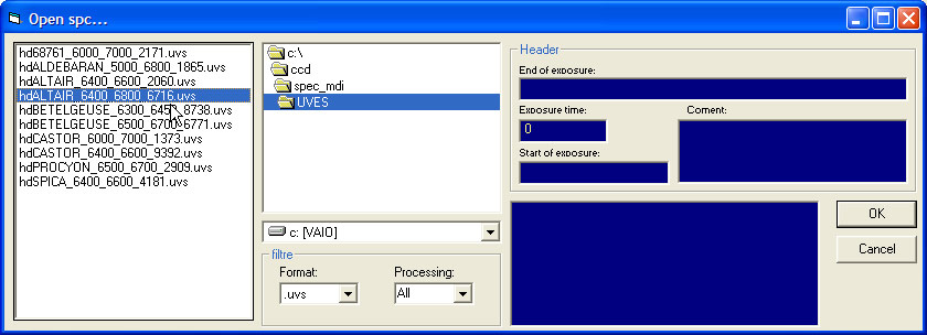
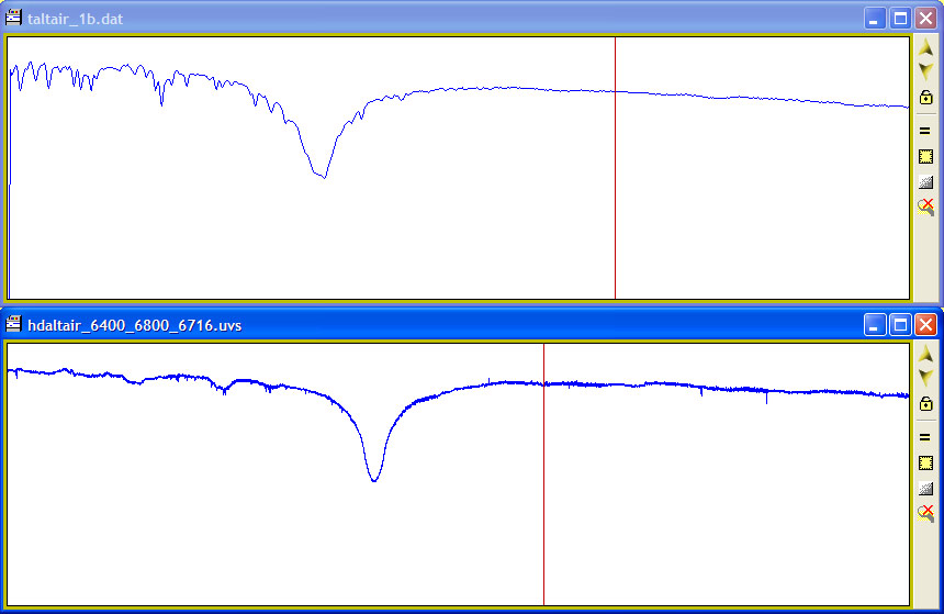
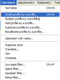
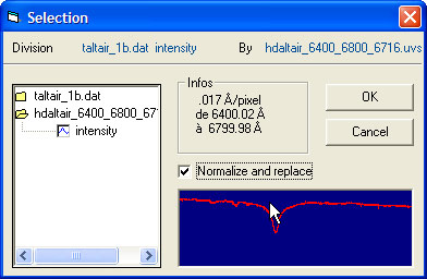
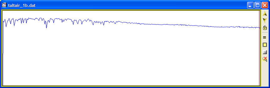
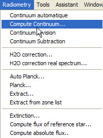
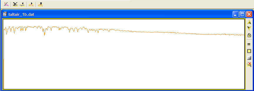
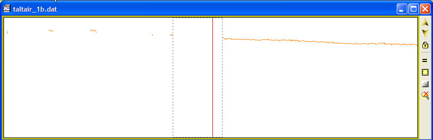
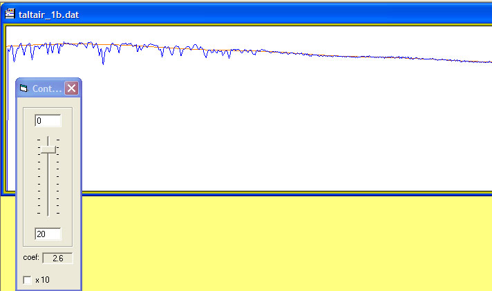
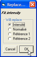
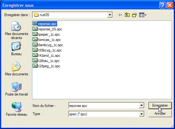
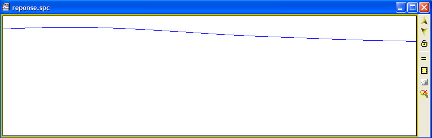
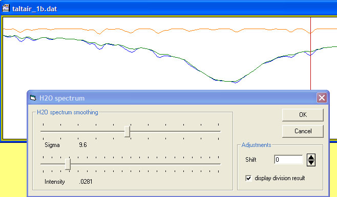
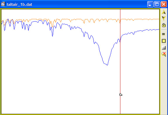
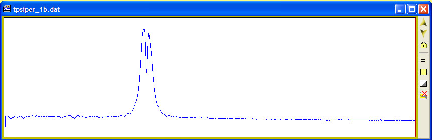
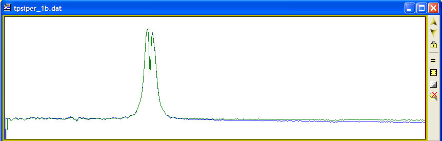
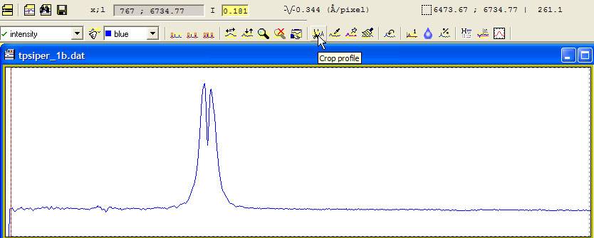
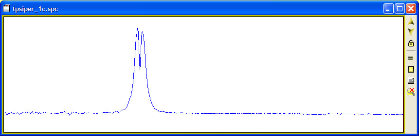
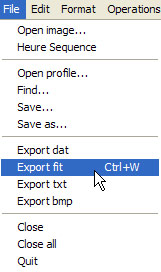
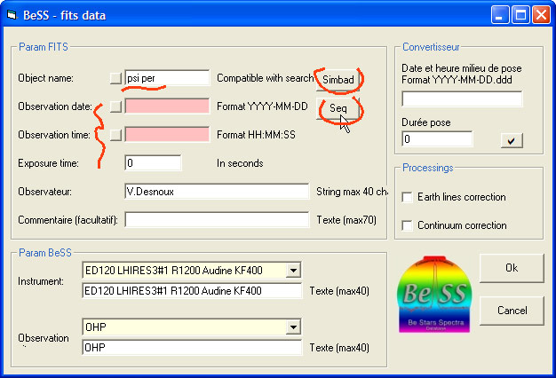
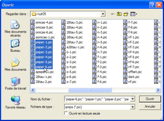
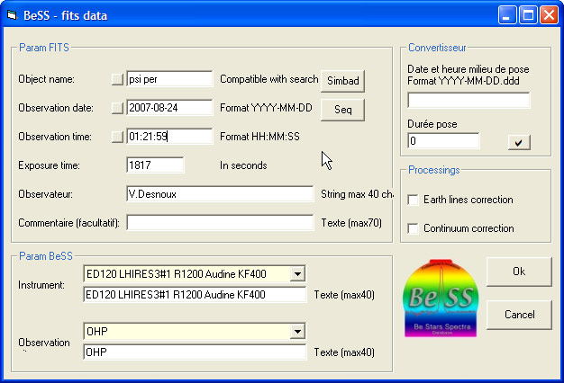
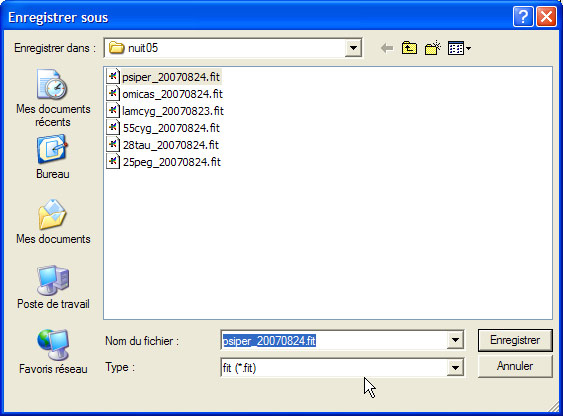
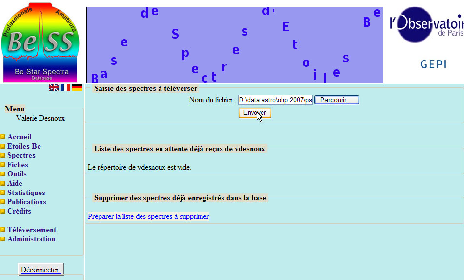
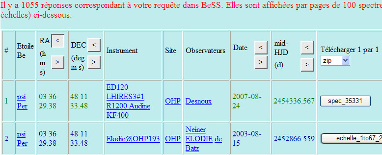
You can download all the files of this tutorial in a zip file: tutorial_ohp.zip Once the star centered in the slit, the sequence of acquisition is of n images of 300sec exposure. The guiding is done either manually or with auto-guiding, with a watec 120N on the LHIRES guiding port. The software used for acqusition is PISCO. The number of images in the sequence depends on the magnitude of the star. The exposure time shall be checked to not have a saturated line in the spectrum. 6 images have been acquired. At the end of the sequence, a spectrum of the neon lamp as the reference for calibration have been acquired. It has to be noted that preferably a neon spectrum shall be acquired at the beginning and at the end to check if there was no shift during the sequence acquisition. The shift would not be due to guiding, but to relative shift of elements inside the spectrograph relative to the slit. In our case, as we found the configuraiton quite stable, only one reference neon has been taken. The acquisition is completed, one can move to the next star in the list. But for the later processing, the following set of images havae to be recorded during the night: - offset images, was 7 images of zero length exposure - dark images, was 7 images of dark image at 300s exposure - flat images, was 9 images of flat images & dark images at the exposure length of the flat The flat images The flat in spectro are intended to primary correct the local brightness non-uniformity of the images. Can be due to dust, pixel to pixel gain, slit... A very detailed analysis of the flat in spectro imaging made by Christian Buil can be found here. The flat set-up consists in using a powerfull white incandescent lamp, placed at the front of the telescope. The telescope entrance is covered by a tracing paper. The exposure length is determined to have the dynamic of the sensor around 2/3 used to increase the signal to noise ratio. The reference star During the processing steps, the instrumental spectral response shall be computed to correct the influence of the sensor on the relative intensity of the spectrum. To do this, a spectrum of a "reference" star shall be acquired during the night. Reference star are well-known bright star, for which we can find a spectrum profile on the net already corrected of the instrumental effect. They also be of a spectral type which does not have too many spectral lines. A-type stars are often selected. In this case, Altair has been used as the reference star. All the images required to fully process the spectrum are now acquired. Two steps will follow: images pre-processing and profil processing. We will benefit of the automatic function of Spiris software - this freeware is a special version of Iris dedicated to spectral processing. In near future, Spiris may disappear and all features will integrated in Iris. Before processing star spectrum The dark, offset and flat images shall be generated. - offset: median sum of the 7 images, produce offset image - dark: median sum of the 7 images, produce dark image >find_hot cosme 400 cosme will be the name of the file which contains the pixels to be corrected by ots neightboors, 400 is the threashold above which the pixel intensity will be tested - flat: dark image at the acquisition time of the flat is first generated, then the flat is computed. Before using the automatic calibration and processing feature of Spiris The CCD sensor is never perfectly aligned with the slit. It can be seen looking at the line of the neon spectrum, they are not perfectly vertical. To correct this geomtric effect (which can also be combined with spectrograph optical distorsion) the angle to correct the verticality of the lines shall be determined. Another paramater to enter in the automatic function is the aprowimative position of the first neon line. This will help the algorithm to automatically calibrate in wavelength the spectrum. Here is the comand sequence (Spiris 1.20) >load apsiper-1 Ready for the automatic spectrum processing We have now all the images and paramaters in hand to automatically generate a 1D profile, calibrated, corrected from offset, dark, flat, sky background, "hot-pixels"... The automatic menu used is the Lhires with a 1200 grating dialog-box This processing will generate the following files: tpsiper_1b.dat - Ascii file with 2 columns: wavelength and intensity - this is the calibrated 1D spectrum of the spectrum Reference star The reference star shall be processed the same way as the star spectrum, with its neon We are now ready to complete the spectrum profile correction and generate the fits file to be load in BeSS Because the calibration has been performed with Spiris, there is no need to do it again with Visual Spec. To complete the processing we first need to correct the spectrum from the instrumental response of the sensor and fill the fits header. Visual Spec preferences Visual Spec allwos to preset the working directory so you do not have to care where the files shall be load from or saved. Always take the time when starting a session to update the preferences. Check the other tab, filling for example the BeSS and position tabs will further helps you in the processing flow. Instrumental response We will first have to find a spectrum of altair fully corrected, on the internet. The database used is the UVES database: http://www.sc.eso.org/santiago/uvespop/bright_stars_uptonow.html The process to load the uvs profile into Visual spec is described in this tutorial. Load here the Altair_uves profile in uvs format, this format is directly readable by Vspec. In Visual Spec, load the altair spectrum from the dat file generated by spiris. Then load the uvs profile The 2 follwowing profiles shall be displayed: Make your acquired spectrum profile the active one by clicking on the dat window Pick the divide profile menu The divide by a profile dialog box appears. Select in the list the profile of the uvs spectrum, to indicates that you want to divide the active profile by this profile. Check the "normalized and replace" box to put the resulting division in the intensity profile. For normalisation, make sure your normalisation wavelength range is compatible with your profile. (In the preference tab). When clicking on OK, the result is the following: The next step consist of removing the residual spectral lines and extract the continuum. For this, we will have to pick the "compute continuum" menu Visual Spec will enter into the extract continuum mode, a new toolbar will be displayed On the profile, with the cursor, click-drag-release around the profile region you want to eliminate from the continuum. Repeat the process on the whole spectrum to keep only region which shall belong to the star continuum. Once done, click on the "execute" toolbar button A new orange serie will be added and a dialog with a smoothing function slider will appear. Adjust the cursor to smooth the orange serie to the best fit of the continuum. Then click on the close box in the slider window. The orange serie will the fit.intensity serie and it is the instrumentale response curve. The last step consist in saving it. Move the fit;intensity serie in the intensity serie. If not done, this serie will not be recorded as it is a temporary serie. Refer to Vspec manual for the detailed explanation. Then save the profile under a new file name, like response You have now your instrumental response curve: You may want to check if Spiris has correctly calibrated your profile. This check is done by the BeSS validators when you submit your spectrum, so why not doing it yourself before. We use the earth atmospheric spectrum with welll-known spectral lines to check if the atmopheric lines of the acquired star spectrum match with the theoretical atmospheric ones. This has meaning only if your spectrum exhibits atmospheric lines. In some observation sites and with special weather conditions, those lines can not be visible or very weak. In this case, the check cannot be performed, you'll have to trust it. Visual Spec use an atmospheric lines list in a special dat file which is provided in your installation package. It is the H2O.dat file. If you have a different file, you can change the pointer to the atmos file in the preference menu, in the atmos tab. Load your dat star spectrum. And click on the button "H20" in the toolbar In the dialog box to adjust the atmospheric spectrum parameter, move the intensity and smooth sliders to best fit the theoretical atmospheric profile (in orange) to your star profile. You can zoom on a region for a better viewing. This does not need to be perfect as you are not going to record the result. The important check is to look at the correct match in wavelenght of the atmospheric lines. You can see in this example that the match is good. This means the calibration is correct. Perform this step systematically is a good practice. On the reference star as well. Instrumental response correction Now that you have your instrumental reponse profile and that you chekced that the calibration is correct, we can perform the correction. Load your star profile, the spiris dat file Load the response profile and divide the psiper profile by the response. You have corrected the profile of its instrumentale response. If you have not checked the "normalise and replace" bix in the divide dialog box, move manually the green serie "division" as the intensity serie before exporting to fits file. It can be appropriate to eliminate some portion of the profile which does not contain relevant data at the end or at the beginning of the profile. This is done using the crop function. Select the relevant portion of the profile to keep, then click on the crop button. Save your result. The save function will prompt you to enter the name of the save file as Visual spec will save it under a .spc format. As a good practice, name your file at this stage with the extension _1c as it has been corrected from the instrumentale response. Exporting into fits "BeSS" format For more details on the BeSS export function, refer to the complement of the user manual here. Load the spc file Export the file as Fits file, compatible for Bess using the menu item export to fit or the short-cut Ctrl+W The BeSS dialog box will appear. Enter the name of the object, here "psi per". The name shall be recognized by the SIMBAD database. Use the button SIMBAD to check on line. Next is to enter the date and the time of the start of the sequence and the overall duration of the acquisition sequence. You can compute it manually or use the new Vspec 3.5.0 feature "Seq". Click on the Seq button. An explorer window will be displayed. Select the image raw files and click "open". Visual spec will read the header of each image, get the date and time, pick the first one and the last one and compute: the date and time of the beginning of the sequence, the duration of the overall sequence. Refer to the BeSS specification here for the details on these paramaters. The result will be displayed in the BeSS dialog box. If the background stay "red", not worry. Complete by picking the right instrument name, observation site and click on OK to save the fits file. Enter an appropriate name. This will be the file that you will upload to the BeSS database, you're done. Go to the BeSS database ! (Before submit your file, may be a good idea to chekc if there are already spectra of this star in the database). Once your spectrum will be validated, you will be able to retrieve it among professional spectra and other amateurs spectra.
This tutorial is based on Visual Spec version 3.5.0 - It shows all the step to go from raw image to 1D corrected and calibrated spectrum ready to be loaded in the BeSS database. The spectrograph used is a LHIRES 3, with a grating of 1200l/mm and a CCD camera Audine with a KAF400 sensor.
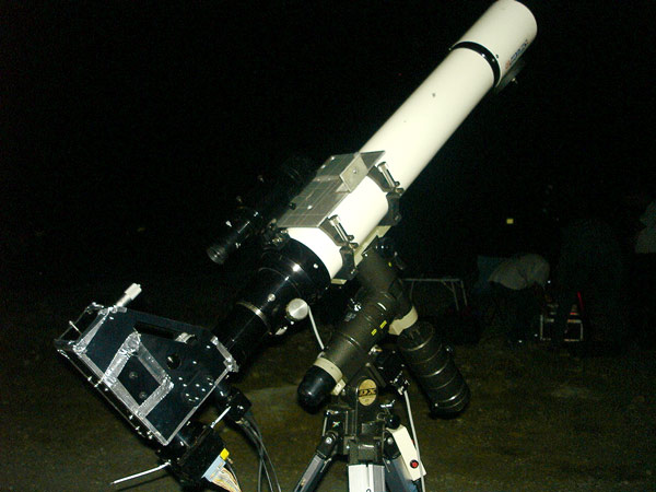
Astrophysic refractor ED120 with LHIRES III spectrograph
Acquiring raw images
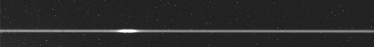
Psi Perseus - raw image of 300s - Be Star, Mag: 4.31 - spectral type B5Ve

Spectrum of the neon lamp - 15 sec exposure - same window acquisition as the raw spectra

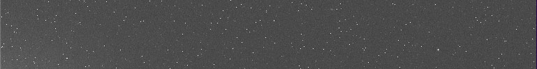
Offset raw image
Dark raw image of 300s exposure
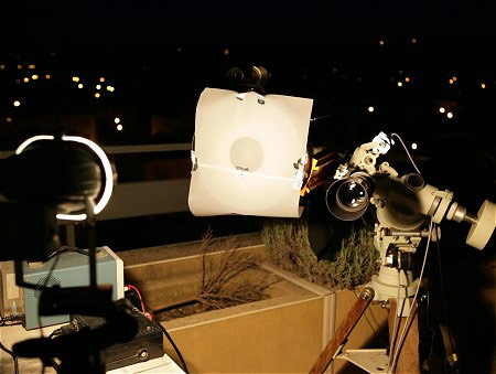
Flat acquisition set-up, using an halogen lamp of 150W - Christian Buil
Raw flat image - 10s exposure

Altair spectrum - 5 images of 120 sec
Pre-processing using SPIRIS
At this stage, it is convenient to also generated the list of "hot pixels" that shall be corrected. On the dark image:
Move the cursor to note the position of the first neon line
>mirrorxy
with cursor, slect the first neon line
>l_ori
Note the angle number which will the slant value correction in the automatic processing dialog-box
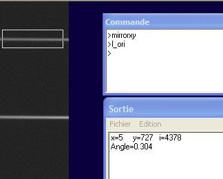
Neon image used to determine slant angle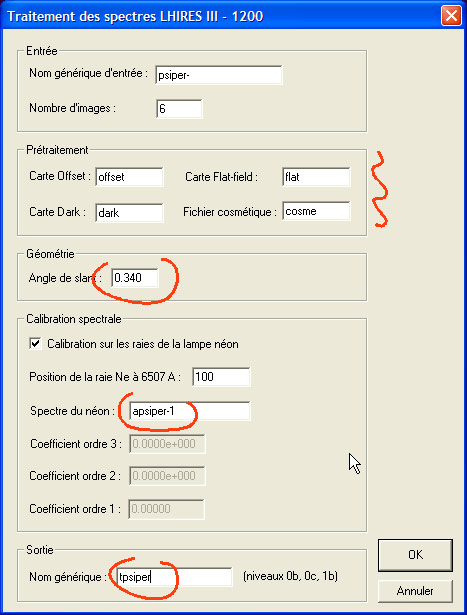
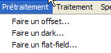
Spiris menu Spectro - sub-item processing of spectra with Lhires 1200
 tpsiper_0b - 2D image of the spectrum pre-processed
![]() tpsiper_0c - 2D view of the binned profile extended to form an image
tpsiper_0c - 2D view of the binned profile extended to form an image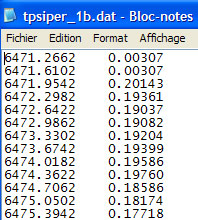

Altair raw image of 120s
Final processing in Visual Spec
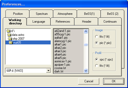
Working directory setting preferences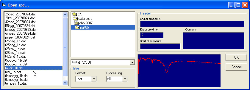
![]()
Checking the calibration
![]()
![]()
![]()