STEP 2 - ASTROMETIC REDUCTION
We will now connect the pixels coordinates (x,y) in image IMG3 with equatorial coordinates (RA, DEC). It is the goal of the astrometric reduction.
Load image IMG3:
> LOAD IMG3
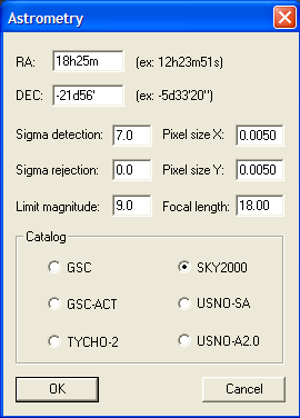
Run the command Automatic astrometry... from menu Analysis:
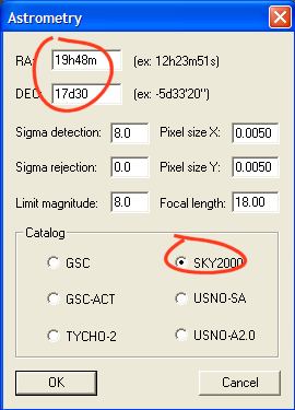
Enter equatorial coordinates of the image center (the same ones adopted at the stage of optical distortion evaluation). Verify that the size of the pixels and the focal length are corrects. Select SKY2000 catalog. Finally, click OK.
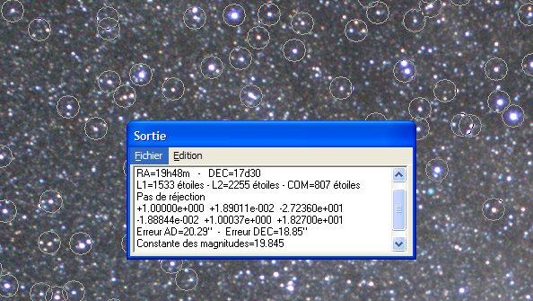
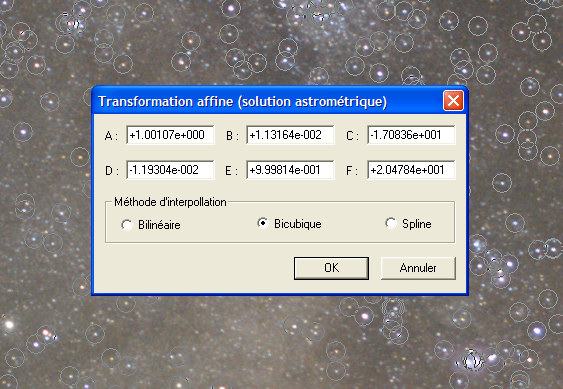
Iris then seeks automatically stars in correspondence between the photographic image and the SKY2000 map. The astrometric reduction is carried out starting from these correspondences. The software surrounds by circles stars used for the reduction. In the output window, the software gives the fundamental astrometric parameters of the image in the form of a set of two equations (one for each axis of the image):
This 3x2 matrix contains the elements of a geometric transformation (translation, rotation, scale) and is read in the following way:
A B C
D E F
The transformation connect a point (x, y) of the arrival to a point (x', y') of the starting:
The parameters C and F correspond to a translation respectively according to axes X and Y.
Normally Iris returns in fact parameters of a matrix of rotation, translation, scale of the form (affine transformation):

In our example we have:
A = +1.00000
B = +0.0189011
C = -27.236
D =
-0.0188844
E = +1.00037
F = +18.270
It will be checked that we have well approximately:
a = A = E
b= -B = D
c = C
d = F
The rotational angle F is connected to the parameters by:


with S a scale factor

The angle is thus given by
In our example, the scale factor is very close to the unit, so we can find the value of the rotational angle with good precision while making simply

The evaluation give -1.08°. a value very similar to your first estimation with Mosaic tool.
Note that the output window also informs us that the astrometrical reduction makes it possible to position the objects of the image with an accuracy of 20 seconds of arc, which is not so bad if the very short focal length the instrument is taken into account (F = 18 mm).
Here, the
software identified 1533 stars in the photographic image, 2255 stars in the
map image produced with catalogue SKY2000 and 807 stars in common. The 807 stars
are used to reduce the image (by the
method of least squares). The correspondance is impossible if the distortion
is not corrected before astrometric reduction!
We will now transform our image IMG3 so that axe X is parallel to the celestial equator and that the scale and the center of image are in conformity with the reduction. Open the dialog box Affine transformation... of Analysis menu:
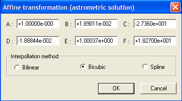
The items are already filled because we have just made the astrometric reduction before. Just click OK. The result the more evident difference is a rotation of 1° approximately. Save the result (give the name ASTRO3 to the file image):
> SAVE ASTRO3
Note: if you made the astrometric reduction from the image ASTRO3 you can note that now the angle F has a null value.
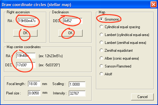
At this stage it is easy to see that the image is correctly reduced. For example identifie the position of the Altair star by its equatorial coordinates:
Alpha = 19h50m47s
Delta = +8°52 '
Open the dialog box Draw coordinates circles... (menu Analysis). Enter coordinates of the star (Altair) and coordinates of the center of the image (always the same ones since the beginning). Also select the cartographic projection. Choose gnomonic projection. Remember, this projection controls the position of stars in photographic images of the sky. Gnomonic projections place the observer at the centre of the celestial sphere and the film plane (or CCD plane) tangent with the sphere at the level of the image center. Its characteristic is that the large circles (celestial equator, declinaison) are lines in the image. Its disadvantage is to deform considerably the aspect of the sky for large field angles (to limit this problem on fisheye lens, the opticians produce a voluntary distortion defect which compensates the proper projection distortion). The fact of having corrected the distortion with precision in our image leads to a nearly perfect projection gnomonic, which authorizes also the astrometrical reduction as we saw. If after correction of distortion no correspondance can be found during astrometric reduction, try to modify values of sigma detection (sensibility to star detection) and limit magnitude of the reference catalog (see Astrometry dialog box).
Click on button OK corresponding to the drawing of right ascension or declinaison circles:
Here the result (a small portion of the image centered on the Altair star):
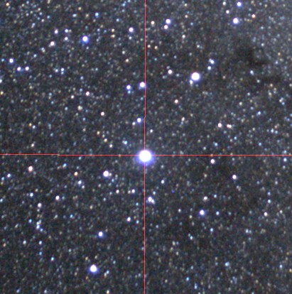
The Altair
star
Another example with the globular cluster Messier 71 in the constellation of Sagittae. Coordinates of M71:
RA = 19h53m46s
DEC = +18°47 '

Identification of
M71 after the astrometric reduction (gnomonic
projection).
The astrometrical characteristics of image IMG3 are entirely defined by the equatorial coordinates of the center, the focal length of the instrument and the size of the pixels. The number of these parameters is restricted, but sufficient. For each image which must constitute for example a panorama it is necessary to attach a specific set of these parameters.
STEP 3: CARTOGRAPHIC PROJECTION
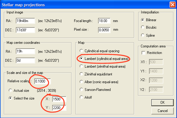
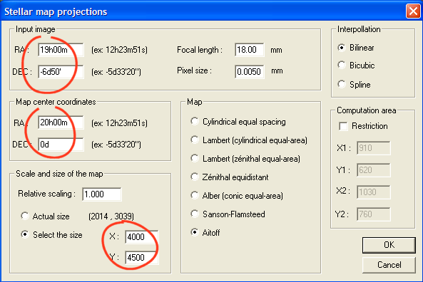
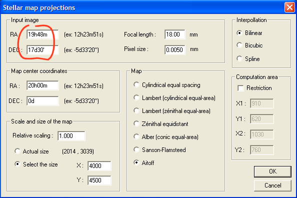
Image IMG3 is defined in a reference gnomonic projection. We now project this image on a cylinder tangent to the celestial sphere globe along the equator. In this projection, the coordinates circles (graticules) appears as a rectangular grid. Right ascensions and declinaisons axis are straight lines. The projection preserve correct linear scale over some portion of the map. It is the simplest map (it is called sometimes Carrée). To proceed, load first the image IMG3 then, call dialog box Stellar map projection... of Analysis menu:
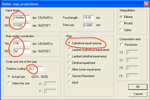
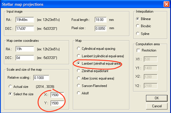
The parameters of the input image concern the starting gnomonic projection. You have to enter the equatorial coordinates image centrer, the focal length of the instrument and the size of pixels. It is all. You indicate the type of card for the result image (output image). Here a simple cylindrical projection. You must then make a decision about the equatorial coordinates which will be at the center of your image at the arrival. In our example the point located at the center of the image will have a right ascension of 19h00m and a declinaison of 0°00 '. Lastly, we define a relative scale factor. If you wish an output image having an average scale identical to the input image, choose value 1.0 for the scale factor. For our example we adopt a factor of 0.2, so that the linear distance between two stars will be reduced of a factor 0.2 between the input and the output. Our field will appear smaller. On the other hand, the size of the output image is the same here as the input (2014 X 3039 pixels). Our input image projected in the new reference map will thus occupy only one fraction of the surface of the output support. Click OK for run calculation.
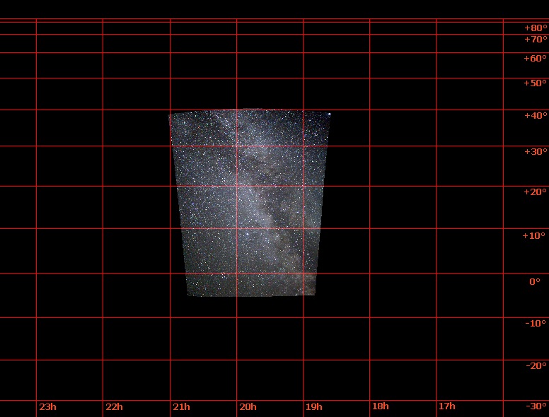
Hereafter, a part of the output image:
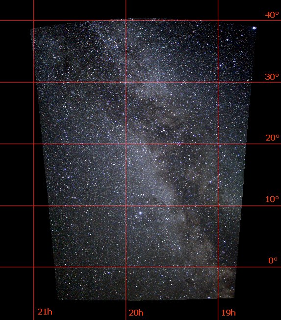
Part of
the image of output. A simple cylindrical projection is used.
The array of coordinates was drawn with the function Draw coordinates circles... of menu Analysis. Note that the grid consists of right-hand rectangles. The indications of right ascension and declinaison were added in the second time with an infographic software (the image is saved before by using for exemple the command SAVEBMP). It is necessary of cource to specify the parameters of the output projection. For example below for the right ascension 20h00m and the declinaison 10°00 ' grids:
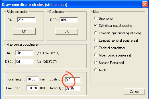
The center of the image indicated is that decided at the time of the computation of the cylindrical projection (19h, 0°). Note, that the scale factor must also be specified in coherence with that adopted during the calculation of the projection (Iris fill this field for you). Define also the correct type of projection (Cylindrical equal spacing).
Taking into account the reduction factor used (0.2 X), a great space around the produced image does not contain information. You can restrict the field of calculation in the output image by define a window (the parameters are the coordinates of two opposite corners):
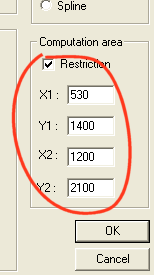
The size of the output image is unchanged. The difference is that calculation is made in the surface of the window which we have just defined. Computation is faster and some alias can be removed.
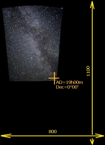
From the Stellar catrography you have also the possibility of defining the dimension of the output image. For example, while making
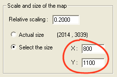
you obtain
We now transform image ASTRO3 (reload it in memory) in a projection known as "cylindrical equivalent " or of cylindrical Lambert ". The cylinder of projection is tangent at the equator of the sphere with radially projected latitudes. An equivalent map maintain constant area scale over the entire surface of the map, an important property for photometric analysis. This preserves the photometric precision when one integrates the signal of a wide source. The polar areas are share elsewhere compressed, which makes it possible to visualize them in a reasonable image of size. For example to make:
The result:
Try now a Lambert's zenithal projection (also know as azimutal projection). Zenithal projections are projections to a plane placed tangent to the globe pole. The point of tangency is either the north or south pole. Right ascensions are represented as radial straight lines through the pole while declinaison latitude appear as concentric circles. Distortion in the map increases with distance from the point of tangency. The projection can represent the entire celestial sphere although it is often limited to showing one hemisphere.
> LOAD ASTRO3
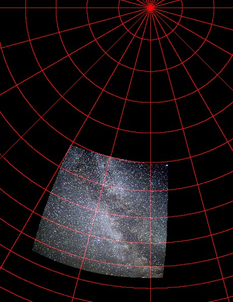
The Lambert zenithal Lambert.
The pole is at the center of the zenithal projection. The surface a preserved (it is an equivalent projection).
In equidistant zenith projection the circles of declinaison of identical steps are spaced by equal intervals in the output map:
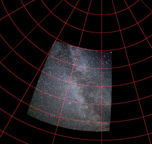
Equidistant
zenithal projection.
In a conical projection, the surface projection is a cone. The cone is placed tangent to the celestial sphere along a parallel of declinaison. Right ascension meridians are represented as straight lines radiating from the apex of the cone and declinaison are represented as concentric circular arcs. Distortion is minimized in a narrow band along the standard parallel and increases with distance from this. The declinaison value of the contact parallel with the cone is the angle Theta. You must enter this angle if conical projection is required. This type of projection is suitable for represent intermediate zones between the pole and the equator with a weak deformation. The Alber's conical projection preserve surfaces. Here an example, with a point of contact of the cone close to the center of the image:
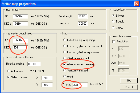
The image ASTRO3 in a conical projection takes the aspect:
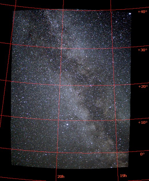
Projections Sanson-Flamsteed and Aitoff are particularly adapted for a total representation of the celestial sphere (there are pseudo-cylindrical projections, more complex than the basic perspective cylindrical projections). The two projections preserve surfaces. Aitoff projection (sometimes called Hammer-Aitoff) distort moderately polar zone. It is a projection very classically used to show global view of the sky.
Example:
> LOAD ASTRO3
then
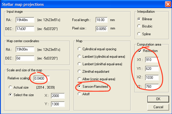
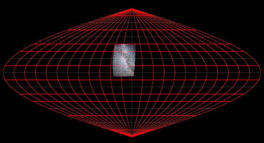
Sanson-Flamsteed projection. Notice the surface covered by
our image
obtained with a 18 mm lens compared to the total surface
of the sky.
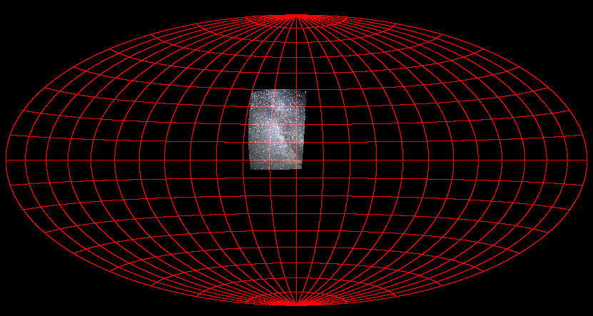
Hammer-Aitoff projection.
STEP 4: CREATING A PANORAMA
The mosaic operation of wide-fields images with a graphic software is a true problem! The connection between the images is nearly impossible because the projection plane change from one image to the another. The optical distorsion is also a serious problem.
The powerful functions of Iris authorise by a simple and rigorous way construction of vast panorama the sky without having to adjust mnually the connection between the images. For example assemble the images FIELD1, FIELD2, FIELD3 and FIELD4.
We have already show how to reduce image FIELD3. The same operations are to be taken back for the three other images.
You must in first correct the optical distortion of each image with the command Correct distortion... of small Géometry menu. You do not have to re-compute the parameters A1, A2 and A3: those found for image FIELD3 apply without problem. The correction of the distortion takes only a few seconds:
> LOAD FIELD1
Call dialog box Correct
distortion and click on
OK without changing the parameters A1, A2 and
A3.
> SAVE IMG1
> LOAD FIELD2
Call dialog
box Correct distortion and click on
OK without changing the parameters A1, A2 and
A3.
> SAVE IMG2
... and so on.
Sequence IMG1, IMG2, IMG3 and IMG4 corresponds to our set of color images corrected for the defect of optical distortion.
You must then consider the approximate coordinates equatorial of the center of each image. For our sequence we have:
Image 1: AD = 18h25m, DEC = -21°56 '
Image 2: AD =
19h00m, DEC = -6°50 '
Image 3: AD = 19h48m, DEC = +17°30 '
Image 4: AD =
20h42m, DEC = +39°54 '
For example, here, the astrometric reduction sequence of the first image:
> LOAD IMG1
Open the dialog box Automatic astrometry... of Analysis menu:
Remember, if Iris informs you that it does not find stars between the image and the catalogue, to modify the value of the sigma of detection (sensitivity to the detection of stars) or the limiting magnitude of stars extracted from the catalogue, then re-run the test.
Continue by the affine transformation (command Affine transformation, Analysis menu):
Finally:
> SAVE ASTRO1
Execute same operations for the other images, the only precaution to take being to modify the equatorial coordinates of the center of the image.
You have now images ASTRO1, ASTRO2, ASTRO3 and ASTRO4.
For example we assemble images ASTRO2 and ASTRO3 in an Aitoff projection with the full resolution for evaluate the quality of the connection.
Load in computer memory the first image ASTRO2:
> LOAD ASTRO2
then
Notice that we redefined the size of the output image. It is very a very large output image so that support can be contain the two projected images in the same representation (the same support) with a center common at right ascension 20h00m and declinaison 0°00 '.
At the end of calculation, the intermediate result:
> SAVE PANO2
Calculate now the projection of image ASTRO3:
> LOAD ASTRO3
We modify only the coordinates of the center of the input image. On the other hand, we do not touch the common center between the images in the output projection (AD=20h00m, DEC=0°):
> SAVE PANO3
For combine images PANO2 and PANO3 you can use the Mosaic... tool (Geometry menu):
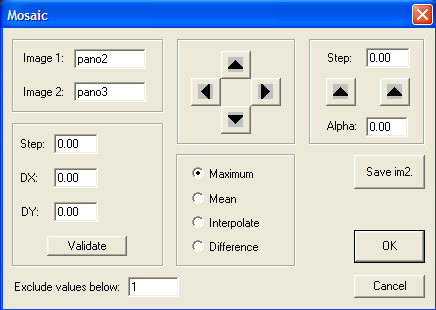
Simply, click OK. you have just completed a panorama containing two great images of the Milky Way.
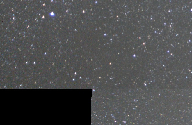
Examine now a small part of images PANO2 and PANO3 in a zone where they overlap:
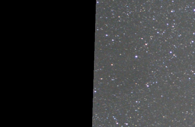
Part of image
PANO2.

Part of image
PANO3 for the same area of the sky.
In the common zones, the two images resemble each other. Only the aberrations of our lens modifies the aspect of the stars (field optical aberration, like coma, astigmatism). The image below is a detail the fusion of images PANO2 and PANO3 for the zone which concerns us:
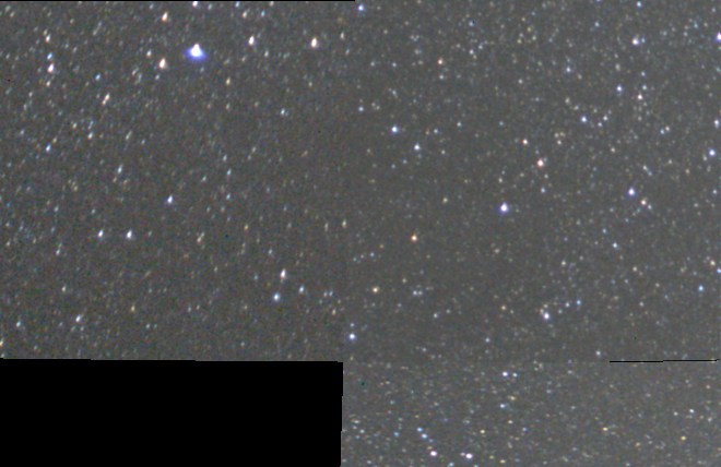
Fusion of images
PANO2 and PANO3.
The illusion which it is about a same image is very good whereas it is about a construction starting from two distinct images. The dark horizontal feature in the right lower part is a traditional problem of edge image (this edge is not clear in one of the images). Command FILL2 can help to erase the part of the images which do not have abrupt edge, i.e. not falling brutally from the nominal level to zero value (filling with zeros of a zone delimited by a selection box with the mouse before run FILL2). Another solution: the command PANO_EDGE is a command designed or clean the border of individuel images of the panorama.
The syntax is
PANO_EDGE [TRHESHOLD]
TRHESHOLD define the intensity of typical pixel just outside the valid image. A small value is recommended (between 0 and 100). Try for example:
>PANO_EDGE 1
Example:
>LOAD ASTRO1
>PANO_EDGE 1
>SAVE
ASTRO1
>LOAD ASTRO2
>PANO_EDGE 2
>SAVE ASTRO2
>LOAD
ASTRO3
>PANO_EDGE 3
>SAVE ASTRO3
>LOAD ASTRO4
>PANO_EDGE
4
>SAVE ASTRO4
It remains your responsibility to harmonize the level between the images so that the connections occur without effect of staircase. This passes by a rigorous preprocessing of the images (in particular the flat-field correction) and perhaps the use of estimation of the sky background (see here for example).
The fusion of
images PANO2 and PANO3 after the use of PANO_EDGE command.
It is instructive to produce a voluntary shift of 3 pixels along the horizontal axis between images PANO2 and PANO3 then to merge:
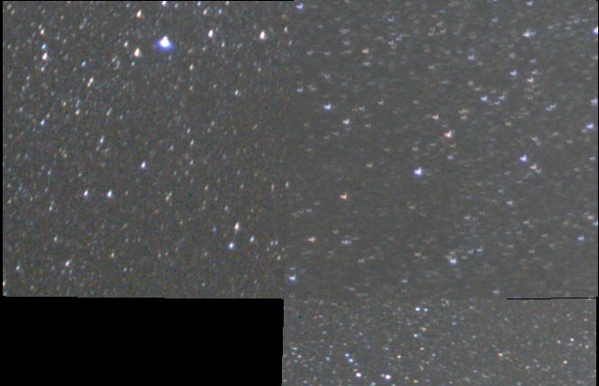
Images PANO2 and
PANO3 with a horizontal accidental shift of 3 pixels.
The effect is immediately visible in the panorama with the junction of the components. The optical distortion present in the original images represents more than 10 pixels in some n parts of the field. The initial errors of projection between the elementary images can reach 20 to 30 pixels. One conclude all the importance to have corrected the distortion and the interest to have a common reference projection for the images.
For assemble a sequence of image you can use the tool Mosaic, while proceeding two by two images. You can also use commands PANO_MAX and PANO_MEAN. The first command merge the images by preserving only the pixels of maximum intensity in the zones of recovery (it is a this function which used here because the connection in intensity is not perfect in the sequence, and PANO_MAX tends to attenuate these defects). PANO_MEAN average intensities in the zones of recovery. The null or negative intensities have a particular importance: they are not taken into account during calculation. For example let us suppose that in a zone of recovery we have for an image the intensity 100 and for another image intensity 0 (because the image is not defined in this place of projection). A simple average would give the intensity 50, which does not reflect reality. But PANO_MEAN excluded from calculation the values equal or lower than 0, so the finally calculated level is 100, which is close to reality.
The syntax of the commands of fusion is:
PANO_MAX [NAME] [NUMBER]
PANO_MEAN [NAME]
[NUMBER]
NAME is the generic name of the individual images of the panorama. NUMBER is the number of elementary images.
For example, for our example we can make:
> PANO_MAX PANO 4
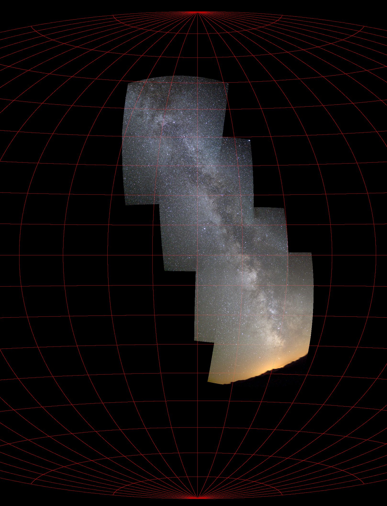
The final panorama by using equatorial Lambert projectiont (the equatorial coordinates of the center of the panorama are (AD=20h, dec=0°):

Click on the image to see a large version.
Below a Hammer-Aitoff projection (we can appreciate the surface covered compared to the total surface of the sky):
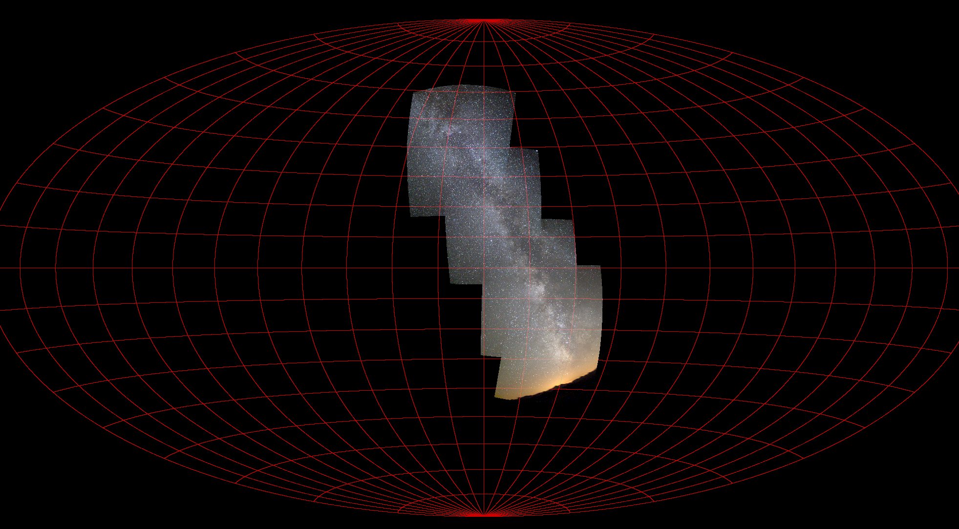
Click on the image to see a large version.
A detail of our Hammer-Aitoff projection, which shows the effectiveness of this one to visualize a wide field without an excessive deformation of the constellations:
Click on the image to see a large
version.
BACK NEXT GO TO IRIS INDEX PAGE