
Comparative
display of a spectra sequence
Cliquez
ici pour une version en Français de ce texte
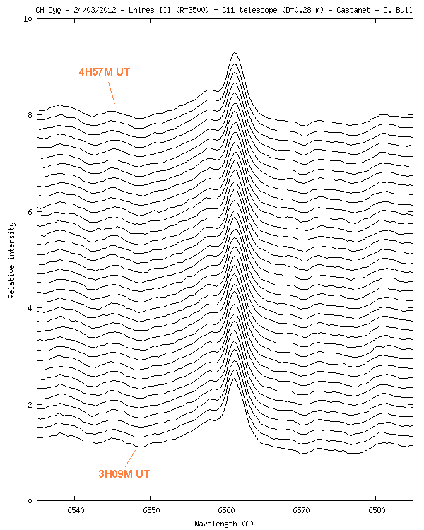
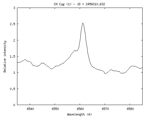
Astronomical objects observed with a specrograph are often highly variable on time scales ranging from seconds to years. The ability to view these variations is of
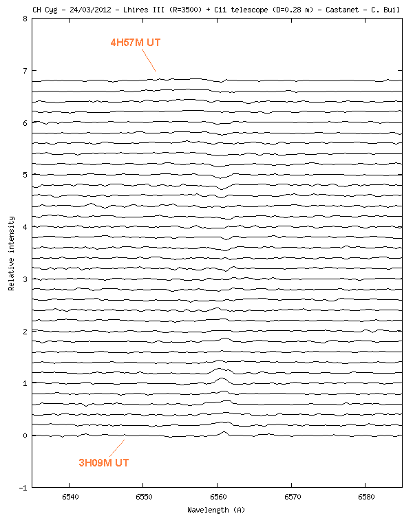
first importance to assess and interpret phenomena. The following figure shows for example the time evolution of the star CH Cyg over a sequence of 35 spectra acquired March 24, 2012 with a time resolution of
the order of 3 minutes
:
This page explains how to produce the effect of this figure with the help of the ISIS software. First a word about the processed
spectra treated. The aim was to measure the appearance of the Halpha line in support of a space observation
carried out simultaneously. The spectrograph is a Lhires III, equipped with a 600 lines/mm grating,
mounted on a Celestron 11
telescope. In the graph, we have an offset of 0.2 units in intensity between successive spectra
to clarify the display.
Here the sign "General" completed for the treatment of this sequence spectrum of the star CH Cygni:
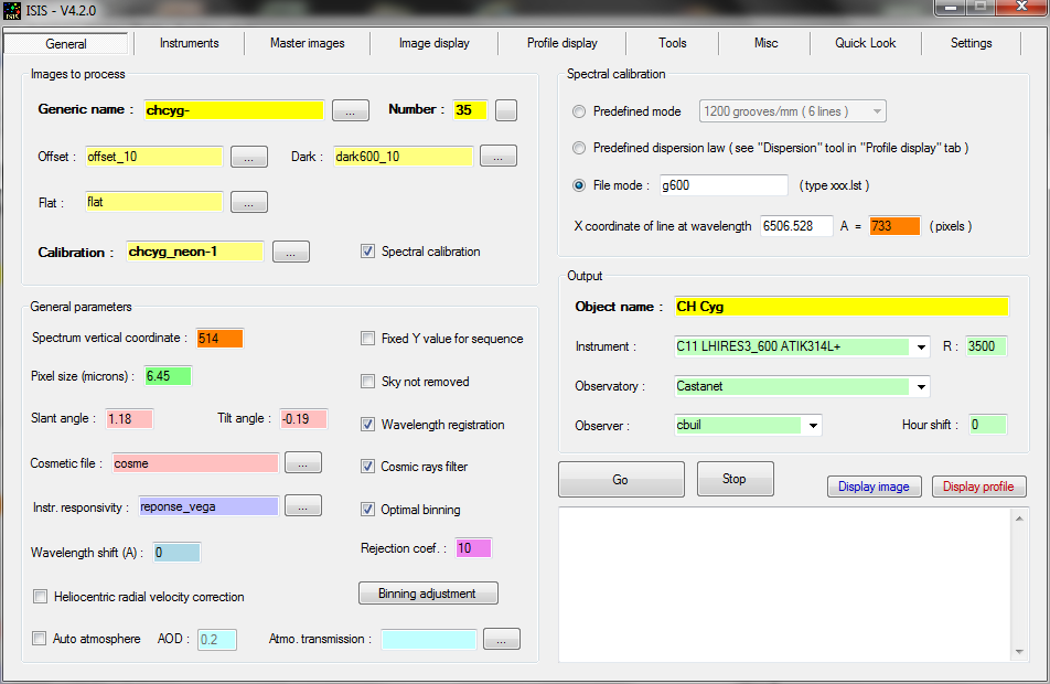
The name of the images is chcyg-1, chcyg-1, ..., chcyg-35 (followed by the extension FIT or FITS). The calibration file is an image of the spectrum of neon internal
lamp (image chcyh_neon-1).
The slant angles (1.18 °) and tilt (-0.19 °) spectrum were also evaluated (from tools specific to the tab "View Profile".
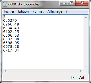
The spectrum is calibrated from a list of
neon lines, whose wavelengths are listed in an external file, g600.lst name (for example).
The first line of
the file indicates the degree of dispersion law
to adjusted, the second line shows the grating
average dispersion in Angstroms / pixel, followed by the wavelengths of lines 8, chosen because they
are intense and islolated):
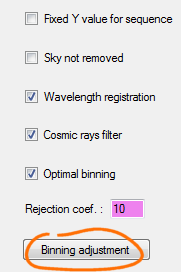
In the "General" tab, note the choice made to minimize noise in the final spectrum: 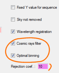
Removal of cosmic rays
option is approved here because the spatial
trace of the spectrum is relatively broad
(warning: the LISA spectrograph that can produce spectra very fine). Detection
cosmic rays
will be effective without degrading the radiometric quality of the spectra.
Note also the use of an advanced feature that allows ISIS to focus the individual spectra in wavelength before adding:
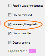
This is particularly useful here because the acquisition sequence is temporally long and the spectrograph Lhires III tends to deform under own weight
(variable over time), leading to a calibration error
If the option is selected, ISIS uses a
intercorrelation method for recenter the spectra, well suited to intermediate resolution spectra. Here in our example,
typical drift during the acquisition (in pixels):
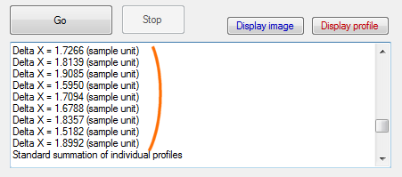
The spectrum image drift between the beginning and the end of the observation is
of 1.9 pixels due to mechanical bending of the spectrograph, which is a lot when attempting to measure the displacement of lines at
a fraction of a pixel.
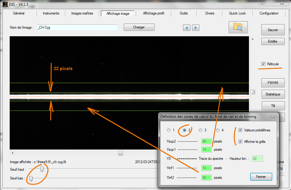
Before starting processing, a good reflex is to verify that the binning width
adopted to extract the spectral profile (including
faint part of the spectrum), but is not so
wide (to maximize
signal to noise ratio). This is a very important check (for
a good job do not hesitate to increase display contrast - after a first
processing run for example):
In recent versions of ISIS you can interactively edit binning and sky
evaluation parameters - the result can be see immediately from the "View image"
tab. Remember to display with
a high constrat:
Now a very important matter for our comparison of spectra: one must ask ISIS to
not delete intermediate files produced after each
processing. Go to "Settings"
tab and select the right option for the occasion:
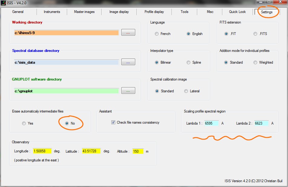
Note for the occasion that we have chosen an area of normalisation
zone in specific to
your spectran, characterized by the absence of spectral lines.
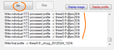
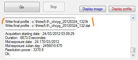
When processing, ISIS automatically saves in
the working directory the spectral profile of our 35 individually spectra. These files always have to name at
this stage : @ pro1, pro2 @, @ Pro3, ...
We will prepare the data to produce the effect of shift plot
introduced at the beginning of this page. This offset is a constant that is added to each profile, with a gradually increasing value as
one advances in time. In practice, use the dedicated "Tools" tab, then "Spectra
processing1"
:
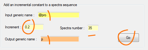
In the example, we produce a shift in intensity of 0.2 units between two successive spectra. The sequence of shifted
spectra is here called p1, p2, p3, ... p35 (arbitrary choice). These
spectral profiles are in FITS format.
Prabably your software is not
capable to plot this format
(Excel for example). So, it is best to convert FITS profiles to
DAT profiles
(simple ASCII files).
ISIS has such a conversion function. Open the "Tools" tab, then treatment "Spectra
processing 3", then finally
:
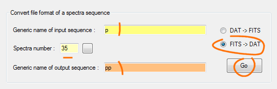
We now have in
the working directory a sequence pp1.dat, pp2.dat, ..., pp35.dat, compatible
with your graph display
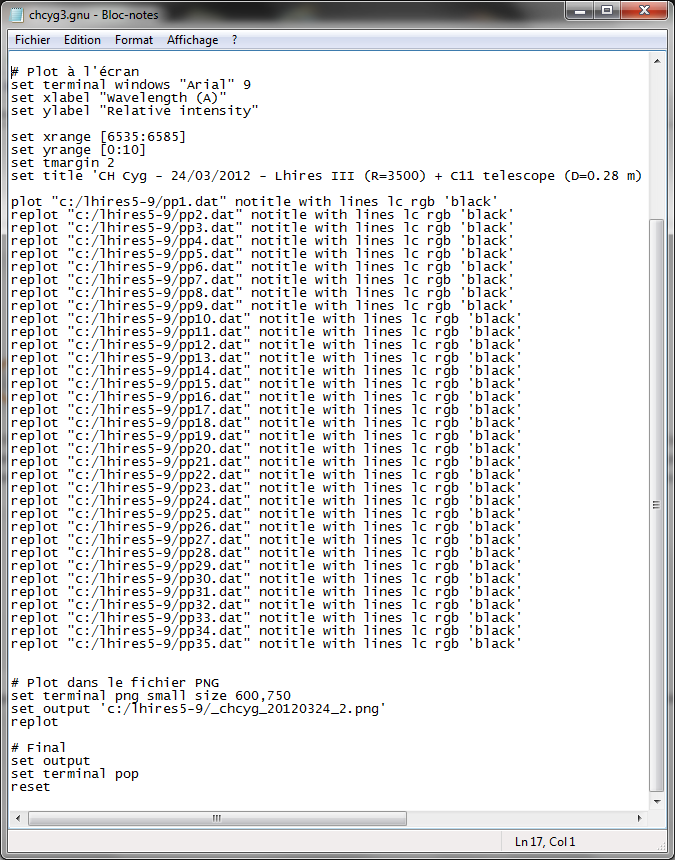
software . Such as gnuplot we can use the following command file
:
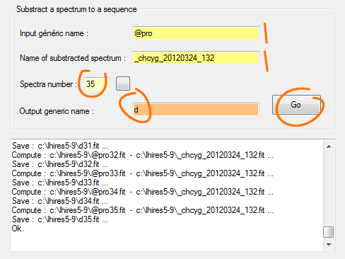
Now we want to calculate the difference between each spectrum of the sequence with the average spectrum of the entire sequence. The result often reveals more subtle variations :
The average spectrum is simply the
composited final spectrum, available at the end of any processing done with ISIS
:
We first calculate the differences ("Tools" tab, then "Spectra processing
2")
:
It remains only to add if desired differences offset
between the spectra :
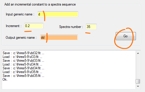
Remember to convert files dd1.fit, dd2.fit, ... in DAT (see conversion function FITS-> DAT, seen above) to view them later as you see fit.
Now we consider to animate our individual spectra to show the changes like a movie. The goal is to reach an animated GIF file, such as:
IMPORTANT: To make an animation, you must first install
Gnuplot free software on your PC. If necessary, see this page, which details how to install this software and configure ISIS. Note that the appearance
of graphic during an animation is controlled by the contents of the Gnuplot
script file called STD.GNU (for example, you must edit this file to change the chart size or adjust the color of the drawing
- see the
installation page).
Since version 4.2.0 of ISIS, synthesis of an animated GIF is considerably simplified. Open the "Miscellaneous" tab then "Animation". Now,
how to complete the animation function for our example:
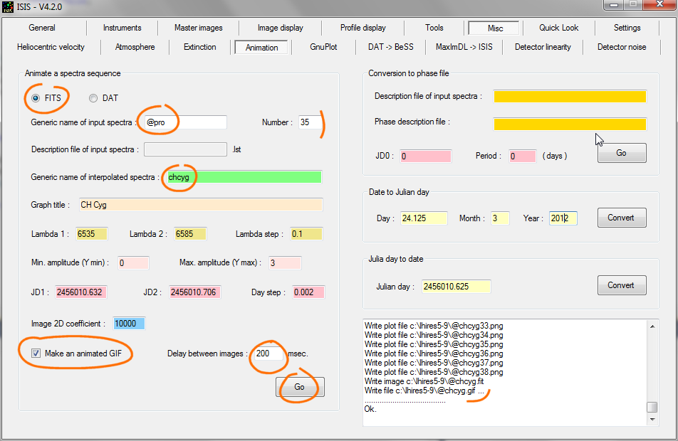
You indicate first
indicate the spectral profiles type to be processed (here FITS format). Then you specify the generic name of these files. We indicate the sequence @proxxx produced
directly after processing of our raw spectra.
Note: the proper spectral calibration is of special importance here. The use of cross-correlation
option at the time of processing often improves the relative calibration between the spectra of a sequence. Sometimes it takes
however, carry out manual editing. For
this use the "Compare" tool
from "Profile displat" tab.
The animation function produces many intermediate files
(by using the generic name "chcyg" in your example). ISIS adds the symbol @ in front of the
files names (this facilitate removing if necessary).
You can give a title to your final graph.
Along
horizontal axis the wavelength interval is fixed by (lambda 1, lambda 2). It is important that these limits are included in the spectral range covered by all the spectra of the sequence (ISIS performs this check). Note the
wavelength step
of 0.1 A selected (ISIS automatically calculates a new interpolated output
intermediate spectra sequence with this step).
The graph shows intensities ranging from 0 to 3 in the example.
The time boundaries are defined in Julian day.
Please note, dates are to be covered by observational data (ISIS can
interpolate data, but it cannot make extrapolation). The selected
day step define the number of images present in the animated GIF. Juts select
a normal time sampling for observe your phenomena. A hundred
image is already a very respectable number.
ISIS synthesizes a 2D image of the temporal evolution. We
give the coefficient used to adjust the intensity of the image (here ISIS multiplies intensity in the spectrum (between 0 and 3 approximately) by 10,000 to transpose the intensity
into the image (the maximum level is
here near 30000 ADU).
We finally select
GIF synthesis option. You can then specify the time interval which will elapse between two images of the film. Here we asked for a time of 0.2 seconds.
The result file (chcyg.gif) is in the working directory.
Back
|