ISIS
Version
5
Guide
for process Alpy 600 spectra
1. Purpose
This tutorial concern profile extraction of spectra taken with Alpy 600 spectrograph.
Important: The processing procedure is very similar to that used for the LISA spectrograph (see here the LISA tutorial). I described here only the main differences.
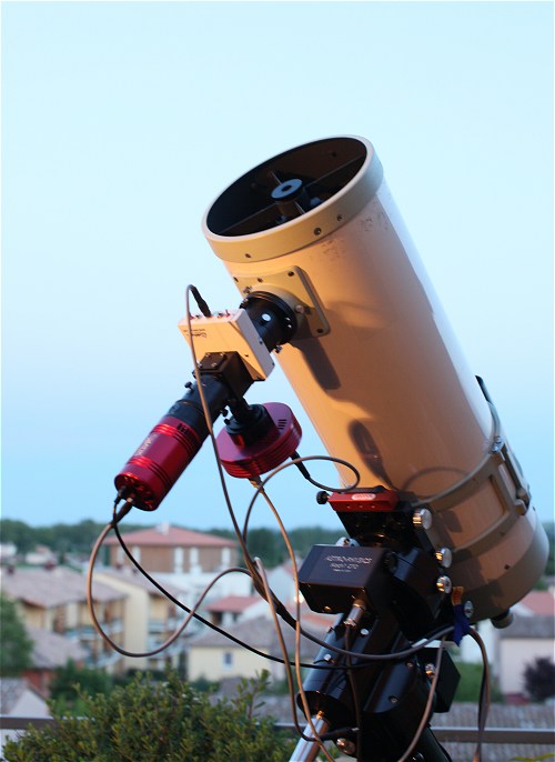
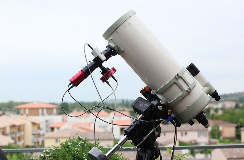
We process a sequence of 8 spectral images of star HD192640 (type A2V, a MILES star present in ISIS reference library). The telescope is a 200 mm f/4 Newton (Takahashi CN212). The camera is an Atik460EX used at its full spatial resolution (binning 1x1, 4.54 microns pixel size).
The data are located in "c:\alpy_tuto" directory (for example !). Here the contain of the main working directory:
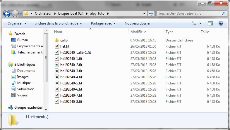
The image "hd192640_calib-1.fit" is a one shot image of Ar-Ne spectral lamp of Alpy 600 calibration optional module (30 to 60 seconds exposure). A method for calibrate Alpy 600 without the calibration module is also described in this tutorial (section 4).
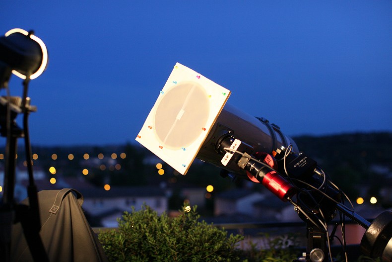
Note the presence of a "flat.fit" image. It is a flat-field image already taken by using the Alpy 600 calibration module (white lamp). You can also use an external halogen in front the telescope + a diffuser (mean of 25 single shots for a maximum SNR - critical, exposed here 3 seconds):
Here the contain of subdirectory "calib":
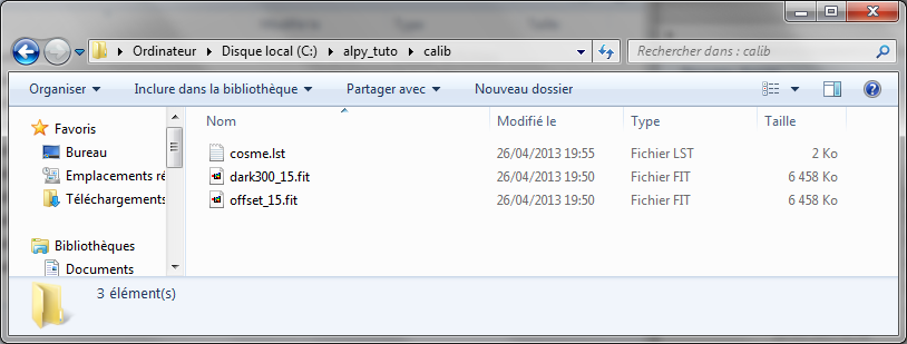
File "cosme.lst" is a cometic file (localization of hot pixels in the dark image). File "dark300_15.fit" is a dark signal reference image (mean of 18 x 300 seconds exposure in darkness). The CCD temperature is -15°C. File "offset_15.fit" is an offset image (or bias image) taken in the same condition (here, mean of 26 elementary frames). Use "Masters" tab tools for compute these reference images.
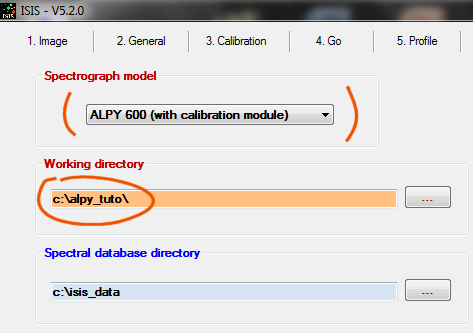
Now configure ISIS from "Settings" tab:
2. Compute spectral calibration equation and instrumental response
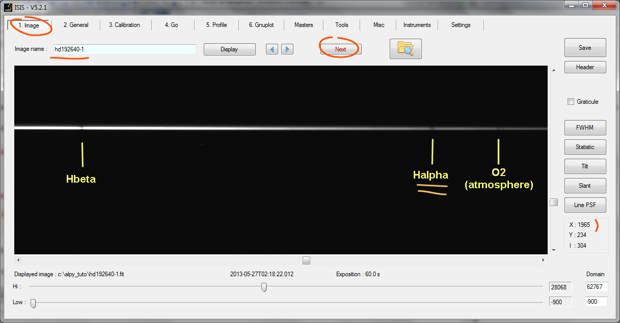
The typical Alpy 600 image of a hot star A2V spectrum (note large and contrasted Balmer lines sequence):
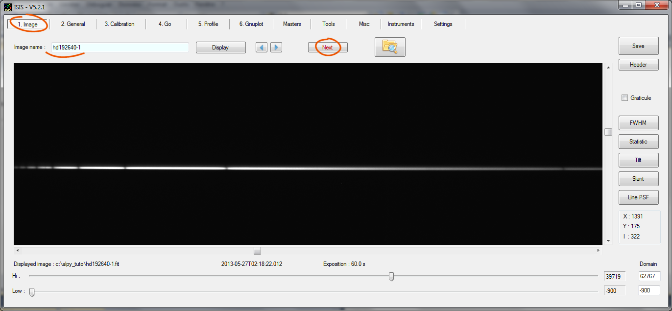
It is the first image of my observational run for the star. Remenber, I use here 1x1 binning for a very well FWHM sampling and for an accurately restitution of the line profiles + minimize radiometric sampling errors.
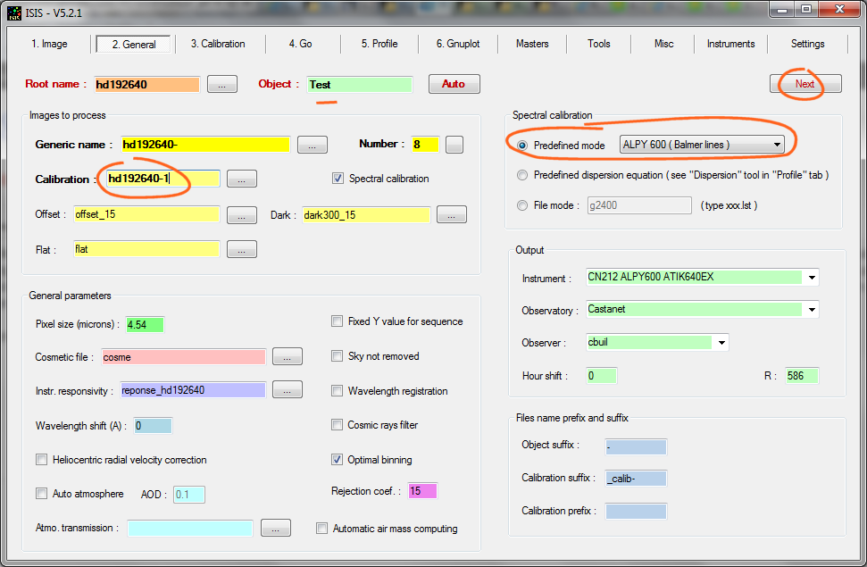
Aspect of "General" tab for compute calibration equation and instrumental response:
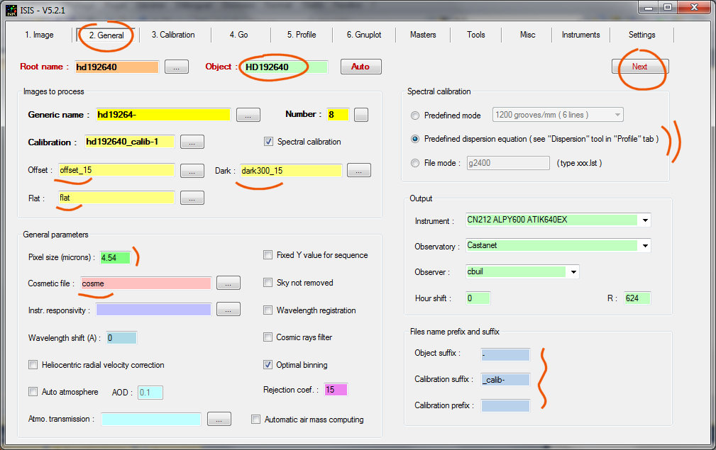
Enter the usual name of the objet, here "HD192640,", then "Next".
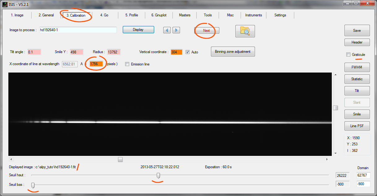
Now the "Calibration" tab :
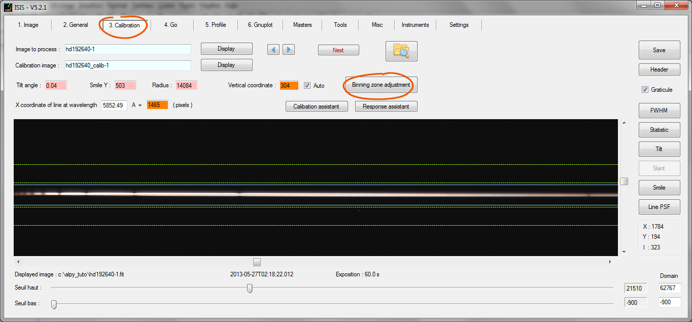
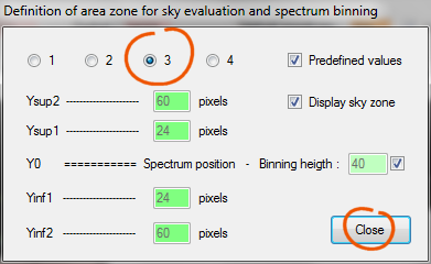
Select a large binning zone because the star is bright:
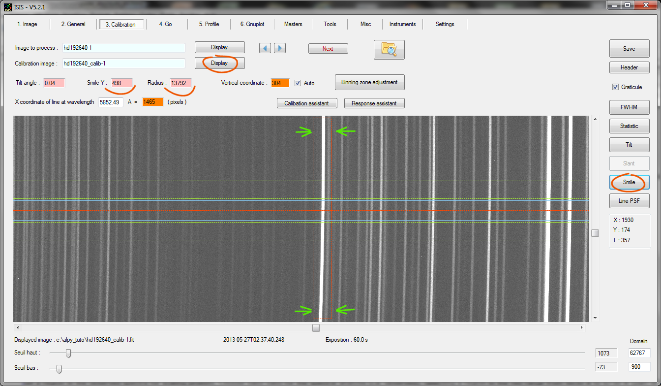
Because presence of some distorsion by the Alpy 600 grism, the spectral lines are curved. It is the "smile" effect. The smile curvature is described by two parameters: the Y coordinate (vertical) of the center of curvature and the curvature radius in pixels. Display the calibration lamp spectrum. Select an intense (unsatrured) line with the mouse over a large part of its height. Click the "Smile" button and ISIS calculates automatically the two parameters:
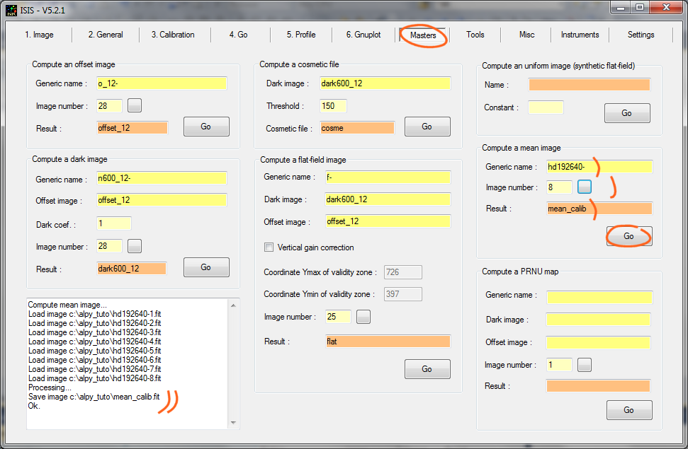
Now, evaluate the dispersion equation:
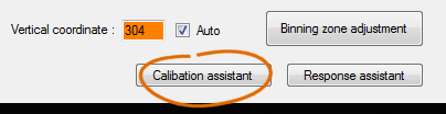
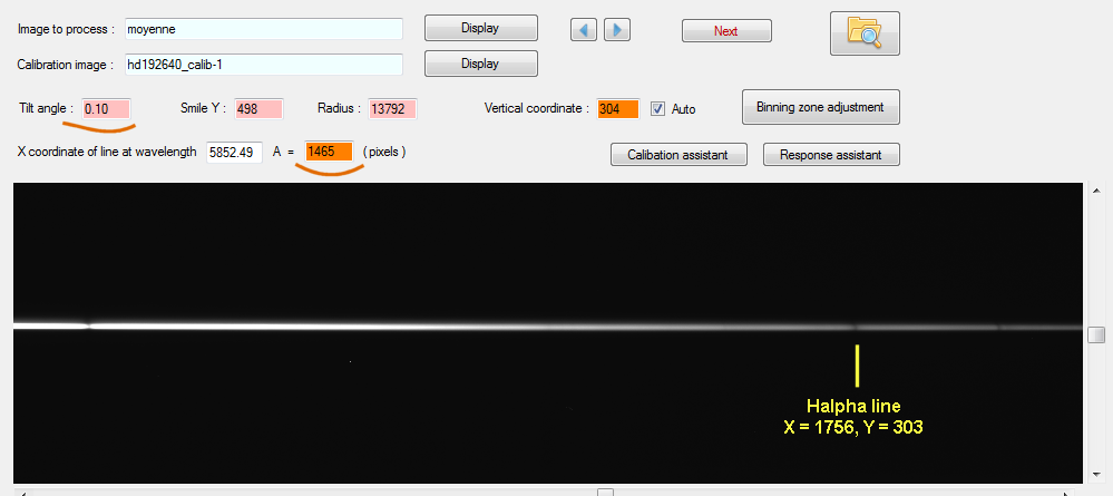
(1) compute a mean image of the sequence. (2) double click with the mouse at the position of Halpha line in image, the fields X, Y for Halpha are completed automatically. (3) click on "Go" button. The calibration equation is computed (4th order polynom) and ISIS return the RMS error, here 0.3 A. All is OK, click "Close" button (with Alpy, max acceptable error is 0,8 to 1 A).
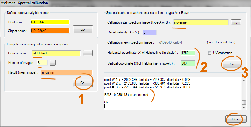
ISIS compute automatically tilt angle of dispersion axis (here +0,10°), and the horizontal position of neon 5852.5 A line (here X = 1465 pixels) :
Note: To densify the number of spectral lines and for maximal precision, ISIS uses here the stellar absorption lines to calibrate the blue part and the spectral lamp emission lines to calibrate the red part. This is the algorithm used by the wizard.
You can see here a summary of methods for calibrate Alpy 600 spectrogaph, from the simplest to the more sophisticated. It is an useful page for help you in many situations.
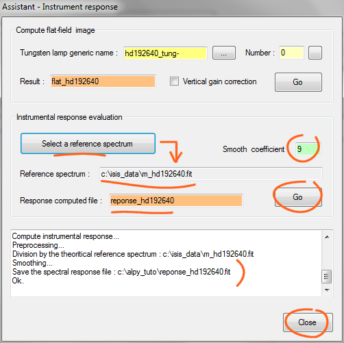
Now compute instrumental response:
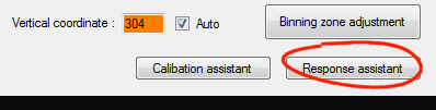
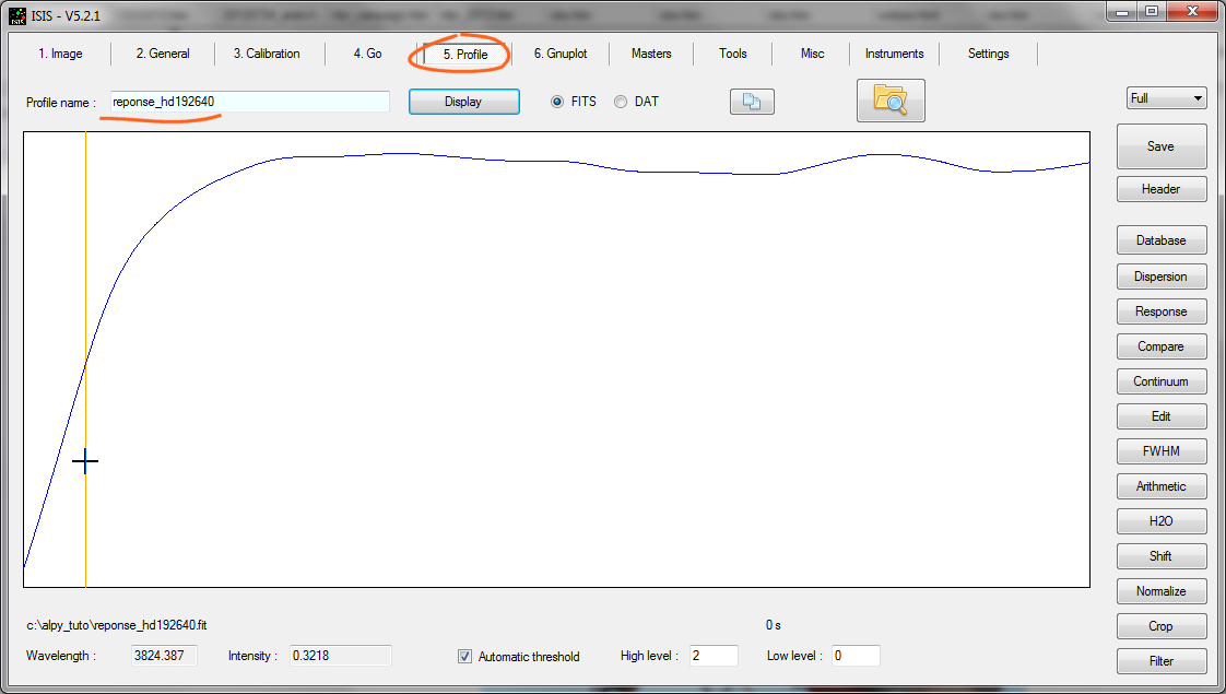
Select HD192640 in the MILES Library. Select a smooth parameter and click "Go". Try and error are perhaps necessary for select the smooth coefficient (see here). Clear lines residues interactively (see LISA tutorial). The name of response file is automatically reported in the corresponding field in "General" tab (here "reponse_hd192640", you can change the name if you prefer) :
The typical aspect of Instrumental Response (RI) with Alpy 600 spectrograph:
See
here a large discussion about methods for compute instrumental
response. The present evaluated response is not the effective instrumental
response because the impact of atmospheric transmission on
the result. It is a pseudo instrumental response.
3. Compute the object spectrum
You are now ready to calculate the spectrum of the star. To do this go to the "Go" tab and click directly on "Go" button. That's all: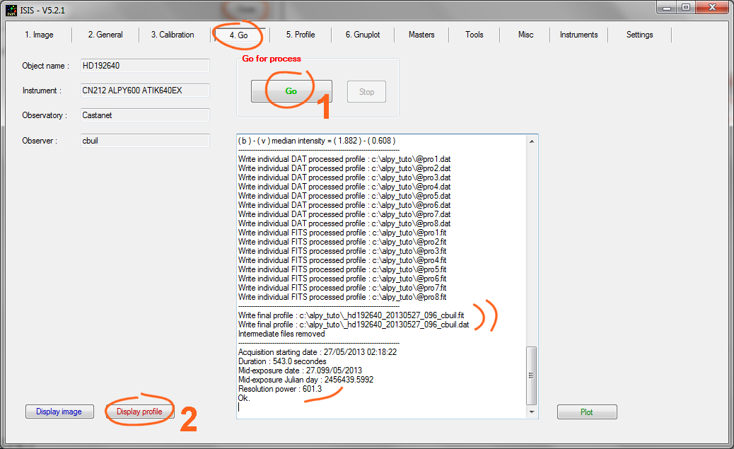
Now display the extracted spectral profile of HD192640:
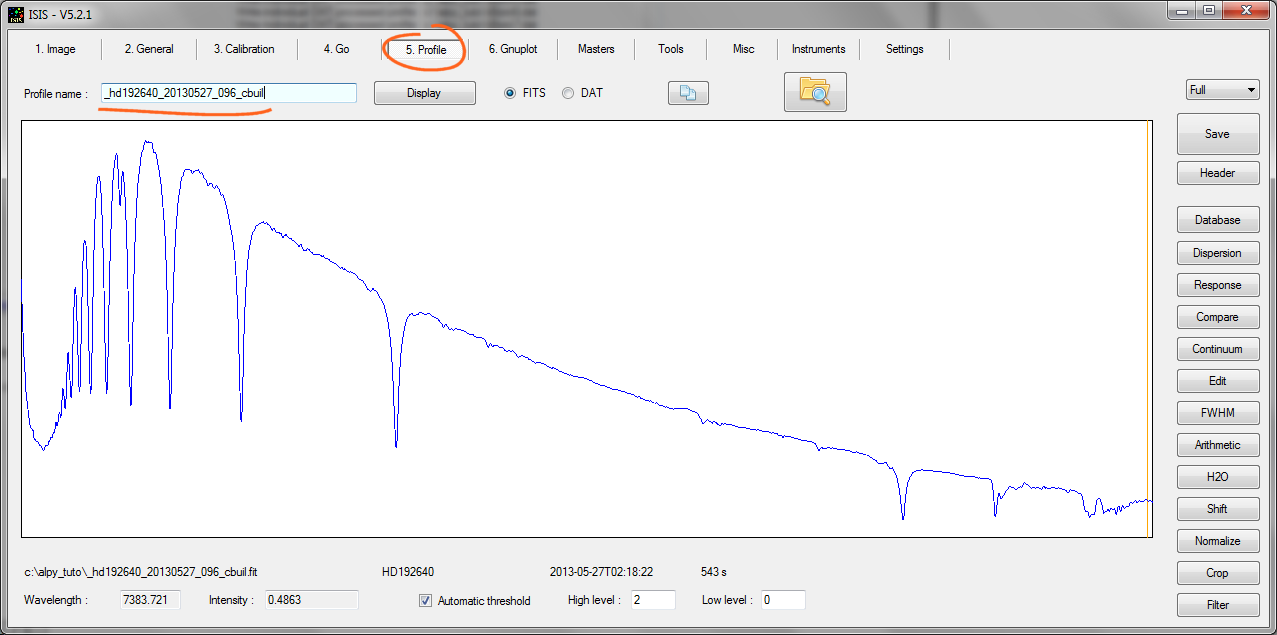
For process a new star, you can
skip the calibration phase if objets are in same area of the sky
(no differential mechanical deformations and same air mass). Enter just minimal parameters in "General"
tab, then "Go" directly.
3. I have not Alpy 600 calibration module !
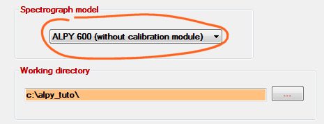
It is easy to find with reasonable accuracy the calibration equation (or dispersion) without having the calibration module. ISIS then used as a calibration source a type A star, in which the Balmer lines have good contrast.First, from the "Settings" tab, select the option "Aply 600 (without calibration module) :
From the "General" tab, in the "Spectral calibration" section, select the Predefined mode, and "Aply 600 (Balmer lines)" option:
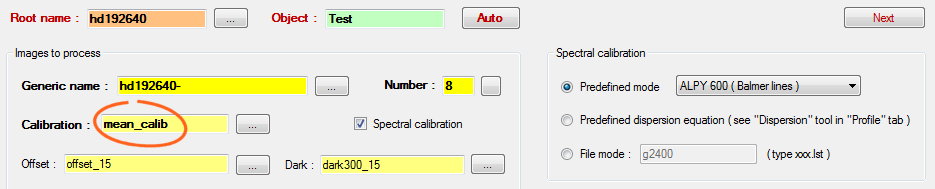
You can also use the average of several raw images computed previously to sometimes improve accuracy, for example :
From the "Calibration" tab, enter the X coordinate of Halpha line:
Note 2: If you are not using the Alpy calibration module system you do not have an immediate solution to calculate the smile parameters. It is recommanded here to use an emission line source with a correct intensity for it. It is possible to use a line of urban pollution, a neon line in front of the telescope, a low consomation lamp (Hg lines), ...).
In the example below, I used a single exposure of symbiotic star YY Her to find the smile from an urban pollution line (it is better to use the mean of available images for increase SNR):
Note 2 : If the camera is properly attached to the spectrograph, smile settings are constants for your instrument!
Now the informations about calibration accurary:
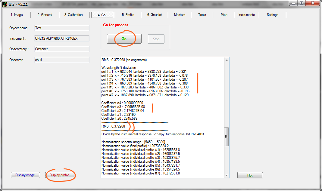
Check the residual calibration error (here, 0.37 A RMS (1 sigma), perfect). ISIS compute here a 3th order calibration polynom by using a limited number of lines (6 first Balmer lines + O2 telluric line at 6872 A).
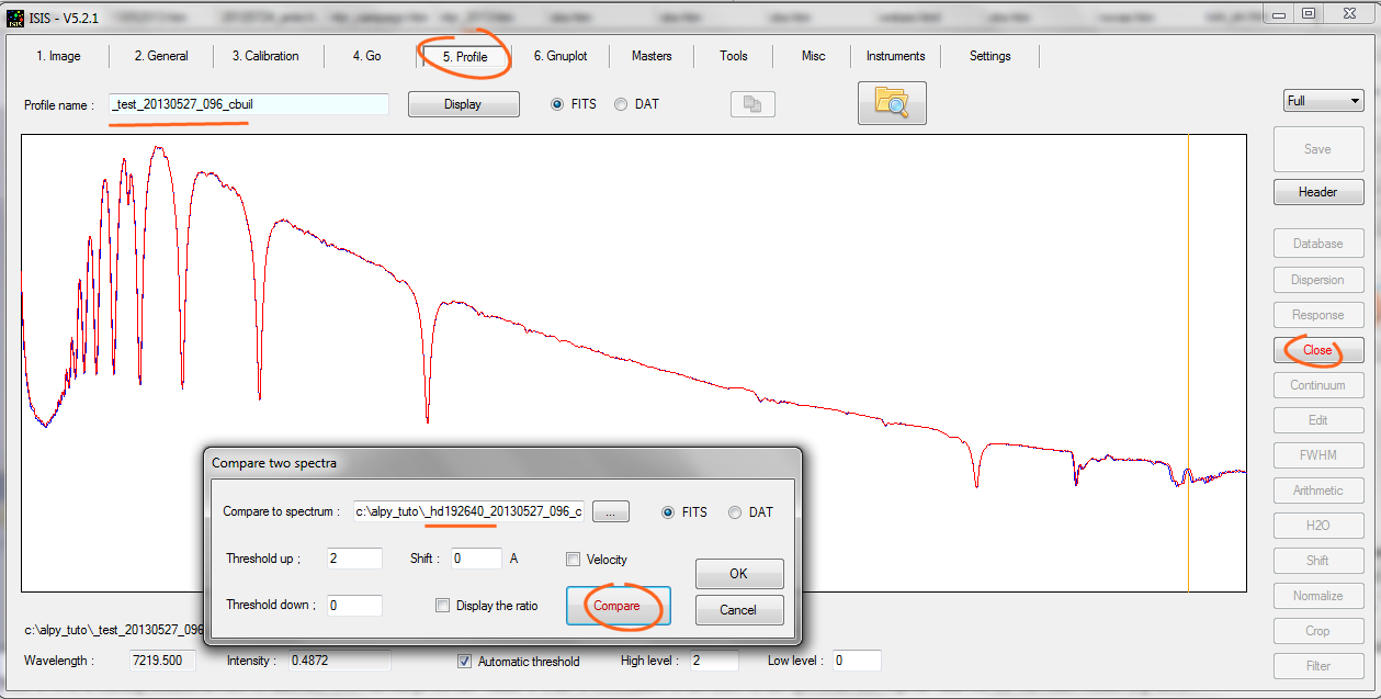
Below, the comparison of the extraction result with the mixed method (star + internal lamp) and the method operates only with Balmer line. In the present situation, the difference is significant only in deep red and far ultraviolet:
Enjoy observations with Alpy 600 spectrograph and ISIS !