14. EXTRACTING THE SPECTRAL PROFILE
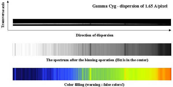
The following figure shows how to extract the spectral profile: the pixels under the star's spectrum are added along the columns (transverse axis). In this manner an image with a single dimension is obtained, the spectral profile. This profile can then be visualized as a graph. For a better interpretation of the profile along the dispersion axis the profile is duplicated along the transverse axis, thus producing a new image with two artificially dimensions.
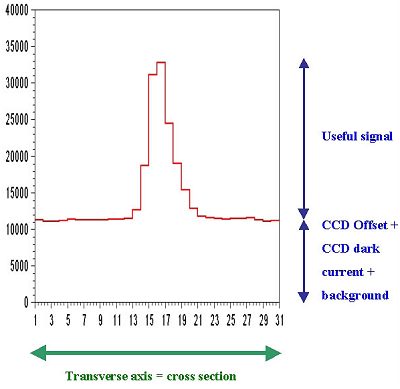
Of course, a spectral image is like any other image: it should be pre-processed first, by removing the offset and the thermal signal of CCD and by dividing by the flat-field image. The following image shows a cross section of a non processed spectrum: note the presence of the sky background signal superimposed on the star's spectrum: it should be removed before usable results are obtained.
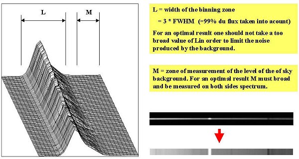
The level of quality achieved in this numerical binning operation has important implications on the final result. If this operation is not properly conducted it may add noise to the spectrum and so limit the radiometric precision. On the following image, showing a spectrum portion in 3 dimensions, the rules to follow are obvious: one should not bin on too large a width L else excessive noise from the sky background would be integrated, but on the other hand L should be large enough that most of the spectrum's signal be taken into account. There is a compromise to be found here. Also the sky background level should be carefully measured on either side of each point in the spectrum, then substracted from the spectrum's value at this point.
Determining the optimal width L is not really obvious. In the following example the blue part of Vega's spectrum (type A0V) is shown. Note that this spectrum was obtained with an Audine camera featuring a KAF-0401E CCD, which gives access to the H and K lines of ionized Calcium below 400 nm (the CaII-H line is practically indistinguishable from the H-epsilon line in this spectrum). The spectrograph that has been used features ordinary dioptric objectives (using classical lenses), there is some severe chromatism in this part of the spectrum, which results in defocusing of the spectrum as a function of the wavelength. Extracting the spectral profile is not very easy, and may imply using algorithms more complex than a mere addition of columns on a given width L.
The following figure shows a simplified algorithm that allows an optimized extraction of the spectral profile. The logics are simple: before summing up the pixels in a spectrum's column, a ponderation proportionnal to the noise's variance is applied to them. In other words, the weaker the signal for a pixel, the lesser its contribution to the line's profile computation. There are several techniques for the weight function W. The one indicated here is relatively simple because the value of the function does not depend on the wavelength. However it is efficient.
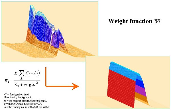
However, improving the signal to noise ratio of the profile R (see next figure) is only significant if the spectrum is very weak. An improvement of about 10% of the signal to noise ratio can be reached, equivalent to a reduction in observing time (for equivalent results) of some 20%. Note that as in deep sky imaging one should composite many spectra to obtain a better signal to noise ratio: this is always the best method for increase detectivity!