OBSERVATION OF THE REDSHIFT OF THE QUASAR 3C273
 

This page presents the observation of a really mythical objects: the quasars.

Note: For a more recent and a more resolved observation click here.

Our knowledge of the quasars comes essentially from the observation of their spectrum, in fact a common denominator for the majority of the objects of the sky. It is by observing the spectrum of the galaxies then, those of the quasars, that the expansion of the universe was established. Their spectrum indeed show a systematic displacement of the spectral lines towards the red, the redshift. This spectral shift is related to a recessional speed of distant objects. It is the famous Hubble law. The speed of recession of a galaxy (or a quasar) is described by parameter z, calculated from the observation of the spectrum:

with Dl is the shift in wavelength of a detail of the spectrum relative to the wavelength l_real, if the object did not move.

The quasar most easily observable is also one of the first discovered: 3C273. It appears as a star of magnitude 12.9 in constellation Virgo (RA=12h29m06.8s, DEC=+02°03'07"). Its z is 0.158 (it is one of the closest quasars - one observes today objects with z greater than 4).

The observation was made with a flat-field telescope of 190 mm at F/D=4 (central obstruction of 0.3), an Audine CCD camera equipped with a KAF-0400 CCD and a Jeulin transmission grating of 100 grooves/mm. The observatory is at Ramonville-Saint-Agne (France, near Toulouse city, suburban location).

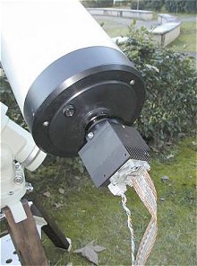
Figure 1. The Audine camera and the flat-field camera 190 mm in diameter. The grating is placed just in front of the camera, inside the filter holder.

The grating is located 19.4 mm in front of the CCD, which gives a dispersion of 45.6 A/pixel (the pixels have a size of 9 microns).

The final image (figure 2) represents the stack of 32 images posed each one 2 minutes. The cumulated exposure time is thus 64 minutes.

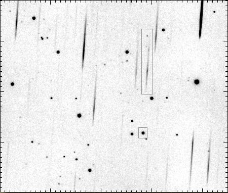
Figure 2. Portion of the final image showing the field of quasar 3C273 (north is at bottom). It is surrounded by a rectangle. Its spectrum is visible at top, surrounded by a rectangle as well. Observation carried out on February 12, 1999.

The value of the seeing influences directly the resolution in a slitless spectrograph. The FWHM measured on the final image is of 2.0 pixels, so that the spectral resolution is 100A.

The spectrum of 3C273 has a sufficient signal to noise ratio to show emission lines immediately. It is already not so bad for a spectrograph costing less than 40 $ (except camera CCD of course) observing an object located 3 billions light years away!

After the traditional operations of preprocessing, work consists in extracting the spectral profile by carrying out a binning optimized over an adequate width in the direction perpendicular to dispersion.

Figure 3. Spectral profile of 3C273 after integration of its significant signal by an operation of transverse binning. Note in addition that the background sky was eliminated.

The calibration in wavelength is made carefully by studying the position of lines of chemical known elements in star spectra observed under similar conditions. Then, the spectrum is re-sampled with a constant step of 5 A/pixel (the software takes into account a possible nonlinear dispersion of the spectrum). In addition I took great care to calibrate photometricaly the data in order to obtain the absolute flux signal coming from the quasar. In figure 4, the vertical axis is graduated in ADU/cm2/s/A. The ADU (Analog Digital Unit) are the steps coders number after the operation of binning. The calibration consists in dividing the signal measured by the collecting surface of the telescope (here 258 cm2, by taking into account the central obstruction), the exposure time (here 1920 seconds) and spectral dispersion (here 45.6 A/pixel).

Figure 4. The spectrum was interpolated with a step of one angstroms per point by using a Spline function procedure, then spectrally calibrated. Moreover, the measured signal was normalized by taking into account of the diameter of the telescope, the exposure time and spectral dispersion.

The profile of figure 4 clearly shows an emission line with 7550 angstroms, another towards 5600A and still another towards 4500A. It is expected in the spectrum of a quasar (see further). However the spectral profile is considerably modulated by the spectral instrumental responsivity and then is poorly related to the actual flux emitted by the distant object. So, to better analysis the data, it is essential to remove the instrumental influence to the raw spectrum.

It is first of all necessary to observe a star for which the spectral distribution flux is well known. The star Vega (Alpha Lyr) is ideal for that, because not only are spectral flux is largely documented, but moreover the absolute illumination, apart from the atmosphere transmission,  is perfectly known (Vega is a fundamental photometric standard). The following spectral profile is the one of Vega star, observed the same night as quasar 3C273.

Figure 5. The spectrum of Vega. The exposure time, 0.3 second, is very short in order not to saturate the detector. One may see lines at 7613 A and 6877 A, which correspond to the molecular center of gravity of the O2 bands of the Earth's atmosphere (telluric bands). The line H-alpha is located at the wavelength of 6563 Á.

The spectrum of figure 6 is artificial. It results from a bank of data which counts relative spectral flux corresponding to almost all the spectral types of stars (Pickles, PASP, 110 :863-878, 1998 July). This tool is very valuable for the spectroscopists.

Figure 6. The relative spectral flux distribution of a standard star such as Vega such as one would observe it outside the atmosphere. Flux is standardized to 1 at 5556 A.

In addition the absolute spectral flux of the Vega star for a given wavelength was published many times (in particular: Tug, White, Astron. & Astrophys. 61, 1977, 679, with an accuracy of 1%). The value at 5556 A is 3.47.10^-9 erg/cm2/s/A (1 W = 10⁷ erg/s). All this information makes it possible to know the absolute signal of Vega on its entire spectrum.

By dividing the profile of figure 5 by the profile of figure 6 one obtains the spectral response of the instrument (which integrates the spectral sensitivity of the CCD, the optical transmission...). But before carrying out indeed this operation it is necessary to take into account that the optical flux recorded with the telescope crossed the earth atmosphere.It is similar to a spectral filter (see figure 7). The operation of complete photometric calibration consists in taking into account the spectral transmission of the atmosphere so that the flux measured by the telescope is just as it would be outside the atmosphere.

Figure 7. Atmospheric transmission for an object observed at zenith. Each curve corresponds to an altitude of observation. Of course the atmosphere is more transparent when one observes from a high place. Absorption is far from being negligible, in particular in the blue part of the spectrum. The atmosphere is almost opaque below 0.3 micron.

Notice that the curves of figure 7 do not take into account the effect of gases of the atmosphere (apart from ozone, O3). The water vapor and atomic oxygen (O2) produce notable absorption bands in the infra-red part of the spectrum. However these bands are local and consequently, it is relatively easy to include their presence during the processing by carrying out judicious interpolations.

Figure 8. The typical atmospheric absorption induced by the gas components. Ozone has effect between 4400 and 7500 A, but it is included in the curves of figure 7. The first serious line is produced by O2 between 6850 and 7020 A, then comes H2O between 7000 and 7400 A, the very significant band of O2 between 7580 and 7750 A and finally, H2O again between 8000 and 8430 A. (according to Fluks & Thé, Astron. & Astrophys. 255, 1992, 477).

To determine the effective atmospheric transmission it is necessary to take into account the zenithal distance of the observed object. If H is the value of the zenithal distance (angular distance between the object and the zenith), one calculates the quantity 1/cos(H), called air mass. Then, each point of one of the curves in figure 7 is put to the power of the air mass. For the present reduction I considered that the observer is located at the sea level. For example, with 5000A the transmission with the zenith is 0.69. The Vega star was observed at a zenithal distance of 50°, from where H= 1.55, and an effective atmospheric transmission for this wavelength is 0,69^1,55= 0,56.

All this mathematical handling and file management is carried out with the assistance of a package of functions especially written for the reduction of the spectral data (namely VisualSpec). The profile of figure 9 shows the instrumental response in ADU/erg, which is similar to the spectral response of telescope + grating + CCD KAF-0400 (warning, each KAF-0400 has its specific spectral responsivity).

Figure 9. Absolute spectral response of the instrument.

For double checking, one can remove the instrumental response to the rough spectrum of the star Vega (division of the last by the first, plus correction of the atmospheric transmission to calculate flux in space). That gives the profile of figure 10, to compare with that of figure 6.

Figure 10. The reduced spectrum of the Vega star (such as it would be observed outside the atmosphere, but without the atmospheric gas compounds O2 and H2O). One notes the continuum which follows the curve of a black body of 14000°K approximately.

The same radiometric calibration is carried out on the raw spectrum of the quasar, which gives the final spectrum of figure 11.

Figure 11. The calibrated spectrum of 3C273. Note that 3C273 is 100000 times weaker than the Vega star.

The emission line towards 5600A becomes now quite visible. One defines its position at 5670A approximately. It was not obvious before the photometric calibration.

The emission line at 7550A is in fact the line H-alpha, which is normally with 6563A for an object at rest. One deduces the value of z :

z = 7550/6563-1 = 0,150

It is a result extremely close to z admitted for this quasar: z = 0,158.

The identification of the emission line at 5670A is more delicate. Initially one can think that it is the line H-beta which is located normally at 4861A. But the corresponding z does not correspond. A bibliographical analysis on the spectra of quasar (see for example Francis & Al. ApJ 373, 465, 1991), reveals in the vicinity of the line H-beta the presence of two lines of ionized oxygen [ OIII ] particularly intense in the spectrum of the quasars (a line at 4959A and especially a line at 5007A, well-known in the spectra of planetary nebulae). In a under-resolved spectrum, the centre of gravity of these lines is about 4880A. z calculated with this value is:

z = 5670/4880-1 = 0,162

If the average of these 2 measurements is made, one finds for 3C273, z = 0,156 + / - 0,015

The identification of the line observed at 4500A is not clear. First its existence is not shown any more in an absolute way on the calibrated spectrum. Then while taking z = 0,158, the wavelength equivalent for an object at rest would be 3880A, which does not correspond to a traditional element in the spectrum of the quasars. Simply, one can say that this line is located not far from the limit of Balmer of the series of hydrogen (3647A). There perhaps it is a group of the hydrogen lines near Balmer limit. An additional observation with a longer exposure time and a darken sky would be necessary to confirm it...

Note that the continuum in the spectrum of figure 11 is completely in conformity with what it is expected from a quasar. Better, the absolute value of flux measured conforms very well with the literature about 3C273. As an example figures 12 and 13 show the spectrum of 3C273 observed with large professional telescopes.

Figure 12. The spectrum of 3C273. 2.5-m telescope Isaac Newton (Palma). Extracted from an article from M.G. Yates & R. P. Garden, My Not. R. astr. Ploughshare, 241, 167-194, 1989.



Figure 13. The spectrum of 3C273 (alias 1226+023). 2.1-m telescope of McDonald observatory. Extracted from an article of K. L. Thompson, A. J, 395, 403-417, 1992.

In these two publications the continuum towards 6500A represents an illumination of 1,5.10^-14 erg/cms/s/A. The present observation gives a result very similar (see figure 11). In the blue part of the spectrum, the continuum obtained with the telescope of 0.19 meter of Ramonville-Saint-Agne follows very closely the one done with the telescope of La Palma (but it is perhaps a coincidence). It may be observed that  the variations can be sensitive between the professional results (see also here).

Conclusion of the experiment: with a grating costing less than 40 $ and a spectrograph buildable in 5 minutes, it is possible in 1999 to measure the expansion of the universe for an amateur astronomer!

Beyond moral satisfaction to observe the redshift of a quasar, you could think that there is no guarantee. You would be wrong! It is necessary to remember under which conditions this observation was carried out: practically downtown, with a lighting which prevents from seeing stars weaker than magnitude 2.5 with the naked eye. Moreover, 3C273 was far from zenith (45° above horizon approximately), which is unfortunately very effective downtown in terms of background sky level. The level of the background sky has a considerable impact on the performances of a spectrograph without slit. Indeed, the background signal is added directly to the spectrum. If the first is very intense, it will scramble the spectrum of the quasar in photon noise. In the present case, the level of the background after binning rises to 371200 ADU, that means a noise of SQR(371200) = 610 ADU, which is considerable. The maximum of our spectrum of 3C273 arrives at level 8800 after binning. The signal to noise ratio is thus only of 8800/610=14. It goes down to 7 approximately at the level of the line H-alpha in the spectrum of 3C273.

A good sky at countryside would give, for an exposure time identical and the same instrument, a sky background of 25000 ADU. The signal to noise is then increased by a factor 4, which could make possible the observation of quasar (or supernovae) down to magnitude 14.5 with a telescope of 200 mm. By using a telescope of 400 mm, a more effective grating and a longer exposure time, I think that it is possible to observe redshifts until magnitude 16.5 approximately. That gives access to a very great quantity of quasars and Seyfert galaxies. Why then not undertaking for example a multispectral monitoring of the variations of glares of objects still so mysterious? To this end, figure 14 shows a standard synthetic spectrum of quasar.

Figure 14. Synthetic spectrum of a quasar compiled by P. J Francis et al. (Ap J, 373, 465-470, 1991). The wavelengths are those of an object at rest. On the left of the doublet Lyman Alpha (1216 A) and NV (1240 A), (towards shorter wavelengths), spectral flux drops quickly because of the gas clouds located in front of the quasar, on the line of sight (many Lyman Alpha lines in absorption, corresponding to clouds of hydrogen of z lower than that of the quasar, result in blocking the light of this last, it is what is called the "Lyman Alpha forest").

You can see on figure 14 familiar lines signatures of quasars: [ OIII ], H-beta, H-gamma...Of course, the line H-alpha, not represented on this figure, remains a very good line to measure redshifts, but when z exceeds 0.5 the line is beyond the wavelength of 1 micron, and it becomes undetectable with the CCD On the other hand, a very intense line like MgII, takes over because it arrives in the visible field. As for the detection of the line Lyman Alpha, its observation with an amateur telescope is a superb challenge, since z has to reach 2.2 so that it becomes visible with a CCD (in particular by using new CCD KAF-0401E from Kodak, with increased sensitivity in blue). There are some quasars between magnitude 16 and 17 which allow such an observation. As for professionals trying to detect objects more and more remote, the visible spectrum can be limited to the only Lyman  Alpha line, the continuum being too weak. But what a beautiful observation! For helping you to identify the lines of your next quasar, the following table lists the major visible feature in these objects, as well as the relative flux which is concentrated there.

Adapted according to P. J Francis et al.

Just do it with your telescope!

(see also the remarkable images of quasars spectra realized by Maurice Gavin).