Figure 1
The figure 1 shows Shack hartmann principle :
A flat wavefront of diameter D1 enters the telescope (or the optical system),
it is depicted by a broad outline, it reaches lens L1, and converges towards
the focal plane, at that point our optical system is completed, so that finished
the telescope part, and that Shack hartmann begins at the focal plane. This
last one starts with a very good optical quality collimator, which turns the
system into an afocal system, it produced a parallel bundles of rays, at this
level the wavefront is again flat. This function can be easily achieved by
an eyepiece, as it produces a flat wavefront reaching our eyes when observing.
Pupil D1 at the entrance of the telescope has been shrink into a reduced D2
pupil. A matrix of micro lenses L3 will be placed on the path, it cuts pupil
D2 into many sub pupils. As the wavefront at the entrance of the micro lens
array is flat, the matrix of micro lenses induces the converging of the light
into a matrix of spotlights, located at the array's focal length.
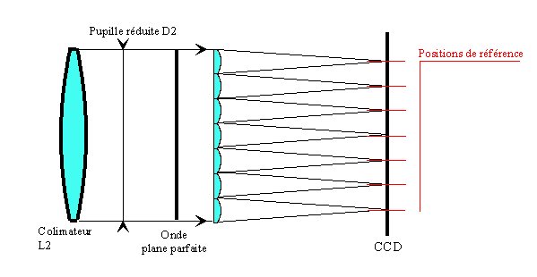
Figure 2
The figure 2, shows, in more details, what's happening at the focal plane
level. The converging beam forms a regularly spaced matrix of spots. The reference
position (X and Y) of every spot on the CCD is measured, thanks to high level
algorithm, the accuracy spot measurement position can be better than 1/20th
of pixels.
If the wavefront at the D2 pupil level is distorted, (figure 3) whether by
optical shape defects ,or by atmospheric turbulence, when going thru the array
of micro lens, the spot position will be changed with respect to the reference
: locally, at the micro lens level, the wavefront is regarded as a flat wavefront,
but at least tilted by a given value. By assembling all these local flat tilted
wavefront that makes the overall wavefront from pupil D2. The measurement
of Dx and Dy distance gap for each spots, with respect to the reference position
found in figure 2a, will provide essential data to reconstruct the input wavefront.
Indeed, Shack Hartmann is measuring the 1st order derivative of the input
wavefront. Wavefront reconstruction is a standard mathematical process, and
is within the reach of modern computers. Wavefront reconstruction is based
on mathematical functions, called Zernike polynomials. This is an orthogonal
set of functions over a circle
having a radius of 1. Other sets of polynomial can be used such as : Seidel
etc… The wavefront can be reconstructed and completely described by
a linear combination of Zernike polynomials Z0,Z1...ZN and their tied coefficients
a0,a1..aN. (have
a look here, for more information about Zernikes polynomials)
Eq 1
- r between 0 and 1
- Teta between 0 and 2Pi
More the Zernike polynomial has higher index, the more it translates to describe
high order aberrations, and thus, more complex wavefront shapes.
This set of polynomial is useful, because they represent optical aberrations that are independent each other. The a1 coefficient in front of Z1 polynomial depicts a wavefront Tilt over X axis which has no relationship with a2 of Z2, the later being a Tilt over Y axis. The a3 coefficient that weights Z3 is regarded as Defocus, that has no relationship at all with a1 and a2. Coefficient a0..aN sets the strength coefficient for different aberrations.This way of wavefront reconstruction using Zernikes polynomials is called Modal reconstruction.
What level of accuracy can be reached ?
This is interesting to compute spot shifts, given a known wavefront deviation : simulations have been achieved .
A pixel size of 5.6µm (webcam pixel) has been considered, a micro lens diameter of 130µm and a micro lens focal length of 5mm. Z8 Aberration, said as 3rd order spherical aberration, has been chosen for this test (revolution aberration)
Figure 4 : Face view of a Zernike 8th, pure wavefront
(3rd order spherical
aberration), in white the positive phase shifts, in black the negative
phase shifts.
No Airy disk degradation is noticeable when Lambda/17 PTV is assumed, which makes a typical spot gap of 0.1 pixels, this is an easy measurement that can be achieved by any image processing software.
| Min Spot gap (Pixels) |
Max Spot gap (Pixels) |
Rms Gap (Wave) |
Peak-Peak gap (wave) Airy |
| -0.05 |
0.04 |
Lambda/112 |
Lambda/34 |
| -0.1 |
0.09 |
Lambda/56 |
Lambda/17 |
| -0.21 |
0.26 |
Lambda/22 |
Lambda/6 (The 3rd ring is enhanced, Strehl
ratio is about 92%) |
| -0.49 |
0.5 |
Lambda/12 |
Lambda/3.4 (the 2nd ring is enhanced, Strehl
ratio about 73%) |
Figure 5 : Wavefront cross
section Lambda/34 PTV
Figure 6 shows spots positions achieved by an highly distorted wavefront
(25 * Lambda) that is going thru the array of micro lens, red dots are
reference spots, white dots are the one measured. This is an actual 600mm
telescope pupil recording. Figure 7 is the computed wavefront. Spots
are missing due to central obstruction and spider legs heavily loaded by cables
.
 Figure 6
  Figure 7
Practical experiments
For experiments, TOUCAM pcvc740K webcam has been used, embedding CCD Sony ICX098BQ featuring5.6µm square pixel size: this a nice, simple and cheap detector, it allows to sample nicely the wavefront variations thanks to its "high" frame rate (30 frames/sec, said fps). An exposure time of 1/300 sec aiming to the Acturus Star, from a 600mm telescope focal plane has been used. The 30fps can freeze somehow the atmospheric turbulence. Collimator optics is an high quality10 mm eyepiece focal length, the micro lens array comes from the Paris-Meudon Laboratoire d'Optique. This is a 22x22 square micro lenses, with a pitch of 130µm and 5mm focal length. This one has been given to me by G.Blanchard : the array of micro lenses is the most critical part in this business, this is not so easy to find, and so spread around nowadays. AMUS in Germany have some for sale, and is making custom designs upon request. I've had, once, a quotation for an array of 30x30 microlens pitch of 148µm and 1.3mm focal length (unfortunately too short) for 300€ each.
The collimator : in that case this is a 10 mm focal length, will provide
a D2 pupil having a diameter of 10mm divided by telescope F/D ratio, i.e.
2.7
mm for F/D=3.7 If one divide 2.7 mm by the pitch of each micro lens, the D2
pupil will illuminate the set of 20x20 micro lenses, this is almost 400 micro
lenses involved: this is a quite good sampling of the incoming wavefront and
allows to figure out high order Zernike polynomials, yielding to high order
aberrations. If a F/16 telescope was used instead, the amount of illuminated
micro lenses would have been 5x5 , which could be not sufficient for optical
tests or optical tuning, but can be enough for turbulence measurements. Shack-Hartmann
parameter design (collimator, size and amount of micro lens and detector used)
depends on application and telescope setup, and cannot be left un computed.
Nevertheless, a different array of microlens can be considered, as well as,
different collimator focal length to be compliant with the telescope F/D and
thus, to get a good sampling of D2 pupil. The collimator optical quality is
critical : if it jeopardizes
itself the wavefront, this is not the atmospheric turbulence that will be
measured, nor the optical quality, nor the telescope optical
tuning defects, but rather the collimator quality or its bad sides effects,
or loss of accuracy .
To prevent from the quality degradation due to the collimator, its mechanical
holder shall be accurately made and a field diaphragm located at the focal
plane will help a lot. This field diaphragm hole diameter shall not exceed
0.5mm, and must be located in the optical axis (CCD - collimator - array of
micro lens). Reference spot measurement using a 5-10µm pinhole at the
collimator focus will be achieved, and afterwards, on sky, the spot measurements
are differential with respect to the reference spot position : this is an
important fact. This means, that if the collimator lens is not perfected aligned
(by fabrication errors), even if the the collimator is not perfect, the benefit
of differential spot measurement (which is the essence of Shack-Hartmann)
will reduce the effect of intrinsic system error, compared to the one we are
about to measure. The key fact is held by the opto-mecanical manufacturing
of various optical element. The separated characterization of the array of
micro lens and the collimator, would be the best solution. Unfortunately,
I do not have the zemax model of the collimator (10 mm Clavé eyepiece).
One should keep in mind that we are using only a 2.5mm diameter pupil compared
to the 6mm needed for the eye, and for which the eyepiece is
optimized. I have made a wood opto mechanical holder, this is not a perfect
solution, and since the results are reaching my expectations, I hope to have
it made of Aluminum soon. The system is a 50x50x50mm cube size, interfacing
to a standard 31.75mm diameter input tube. Such a system is sold by Imagine
Optics, the price is around 40 000€ (!) , mine has, for the time being,
a cost having the same figure with 2-3 zeros less, but mine is not performing
as well as the one from Imagine Optics (professional tool), one should not
forget the software cost developed which is not negligible in this project.
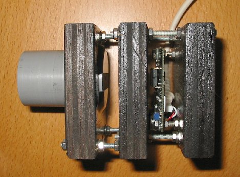
Figure 7a
: This picture is the Shack-Hartmann hardware, right, a webcam board plus
its detector (disassembled for this purpose), the middle wooden block holds
the array of lenses (held by a glass cylinder of 17mm diameter), the collimator,
is also located inside this part. This prototype has been used to validate
the concept and get hands on it.
The fact that the system is not exactly at the telescope focus, is not a real issue, defocus leads to a radial scaling that is applied to the overall array of spots, this will made a non null Z3 (defocus) coefficient : this not a real issue, but must be minimized as much as possible, because Z3 is a defocus approximation by a parabola (this is indeed a sphere).
Figure 8 : Radial expansion due to defocus
To perform the system optical analysis, the 600 single frames (20s) from the
webcam have been stacked. The turbulence effects are averaging pretty well
to cancel out, because atmospheric turbulence (if not so strong) behaves like
a null random variable, provided the acquisition time is larger than 10s,
telescope tracking must be better than one arc sec. To analyze atmospheric
turbulence, frames will be reduced one after each other. This setup allows
two kind of measurements : optical tuning and telescope optical wavefront
analysis, and also disturbed wavefront from atmospheric turbulence : this
is not so bad (!!)
In this test, using the T600mm telescope, the Shack-Hartmann has been installed
behind a Wynne corrector, by nature, this one degrades slightly the diffraction
disk, however, I must say that the field diaphragm was not located at the
optimal distance with respect to the last optical element from the wynne corrector,
i.e. 50mm. A different location jeopardizes the optical quality provided by
the field corrector. Thus, my opto mechanical setup is very useful to get
image data, but to to perform a definitive measurement . The goal
of this experiment made at that date is not to characterize the telescope
and its optical. Rather to acquire data in the goal of writing the software,
and to validate the overall concept was desired. As a conclusion,
the measurements shown here are not definitive and are not showing the performance
of the telescope optics. This is a prototype (May 2003). The day, I could
use a mechanical holder made following the standard opto mechanical rules,
It will possible to make a fine measurement and not a system made of wood
(see next section, because it has become possible in Dec 2003).
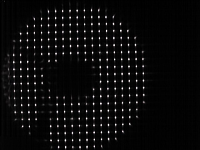
Figure 9 : Shack Hartmann test, T600 Valmeca telescope (Acturus, 1/300s
a 30i/sec)
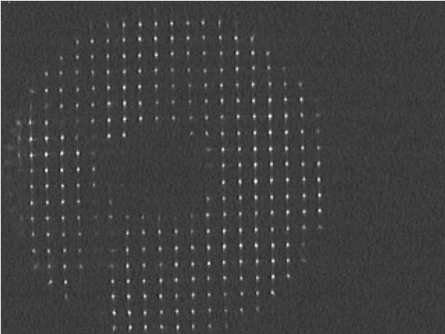
Figure 10 : Shack Hartmann test T600 Valmeca telescope (Acturus, 1/300s
a 30i/sec) Sample frame among 584.
Hereafter the video sequence can be downloaded as an AVI file (584 frames, amazing !) click here to get it (3.5Mo), DivX Decoder is mandatory (get it here). The spots are disappearing because of scintillation and atmospheric turbulence.
Data reduction
This part has requested a lot of programming work to make it efficient and user friendly, it has been embedded to the PRISM software, the first step is to extract the spots automatically and to sort them out (Figure 11). There are 261 spots in this case. The disk shape shows the telescope pupil as well as the central obscuration and the spider legs.
Figure 11, 584 stacked images
The second stage consists in loading an ASCII file that contains the X and Y spot reference position extracted from the figure 2a image. This spot reference data has been achieved by putting a 5-10µm pinhole where the star is located.
Figure 12
Once the reference file has been loaded, the user has to enter to which spot number (#A from image figure 11) matches the spot number (#B from image figure 2b), and some system parameters .
Once the "links" between the spot from the measured image and the one from the reference image are found (automatically), the software can compute the position gaps (DX,DY), and the Zernike coefficients. The DX and DY shifts that affects the whole set of spots between the reference image and the measured image is not important, because it yields to a1 (Z1) and a2 (Z2) which describes only a global image shift, no aberration.
Figure 13 panel shows the a1....a19 coefficients of Zernike polynomials.
The Tilts and defocus coefficient are not enabled, because there are not
optical defects nor aberrations.
Figure 13
Once the Zernike coefficient are computed, they could be modified (or not).At that stage it is possible to compute the point spread function (PSF) that represents the star's image (airy disk image if perfectly flat wavefront). The more the Zn coefficient have high figures, the more the aberration will be visible on the image. As the wavefront is known, PSF computing is possible as well as the Peak to valley wavefront error, as well the RMS (THIS IS A VERY IMPORTANT FIGURE TO CARACTERIZE THE WHOLE SYSTEM).
Figure 14a, b et c , from left to right, star PSF (or image).
14a figure shows star PSF (turbulence has been lowered by summing 584 images), picture 15 is a perfect system PSF. If Z6 and Z7 are set to zero (coma), picture 14b shows the improvement, same operation concerning Z4 and Z5 (astigmatism), the picture 14c, seems to be affected by spherical aberration (this makes sense because the Shack Hartmann was behind a Wynne field corrector). This is very instructive to watch how the PSF is affected by changes in Zernikes aberrations. For instance, this can bring information related to optics stress due to mirror holder and see how effective they are and how to correct it.

Figure 15 Perfect
PSF, same scale as previous PSF images, scale is 0.32µm per pixel at T600mm
F/3.7 prime focus
Effects de la turbulence/seeing
What about seeing ? When the PSF is computed for each of the 584 frames, the PSF is NOT the same from an image to another. Watch the next pictures :
Figure 15 a,b et c : frames 472, 524 et 532
If the frames are averages, the seeing effect tends to disappear. A 600 frame sequence is not to much to do so.
Picture 16 shows 2 consecutive computed frames from the shack hartmann, 33ms
of time gap: the PSF are really different. Turbulence has a low time coherence
scale.
Figure 16 a et b, frames 470 et 469
References
Some papers that helped me a
lot to achieve this project..
- To know all about aberrations theory and
Zernike polynomials
- An Interferometric Hartmann Wavefront Analyzer for the 6.5m MMT, and the First Results for Collimation and Figure Correction
- Interferometric Hartmann wave-front sensing for active optics at the 6.5-m conversion of the Multiple Mirror Telescope
- Zernike polynomials (maths)
Thanks to G.Blanchard, S.Guisard, A Maury and S.Deconhiout for correcting this page and the help brought for this project.
By Cyril Cavadore
(December 2003), Back to Home Page