Once the first tests passed successfully, new mechanical parts
have been designed and manufactured to get a better optomechanical setup.
This will allow fine and actual measurements. Those parts were manufactured
by the help of F.Colas and M.Meunier.
The following pictures shows how it looks like (like a camera
indeed) :

(figure 1) This is the complete Shack Hartmann setup, aluminum casing,
31.75mm input diameter.

(figure 2) The detector compartment, this is a TOUCAM PCB webcam,
embedding a 640x480 5.6µm pixel CCD read out at up to 30frames per second.
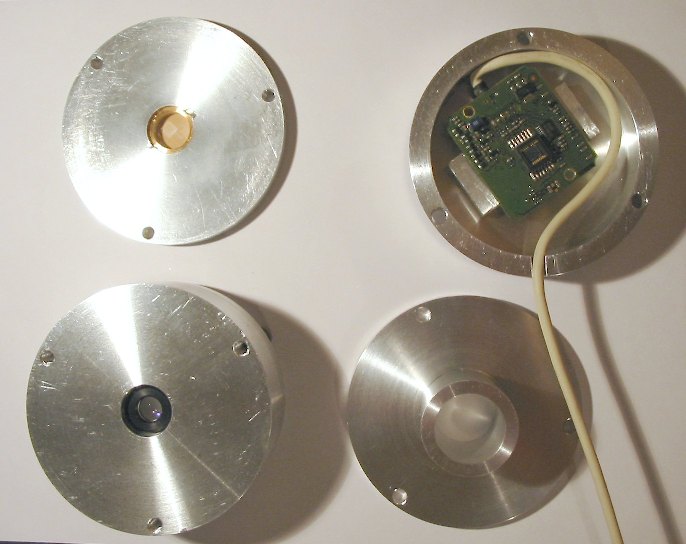
(figure 3) All the system disassembled : top-left the microlens holder,
bottom left the collimator,
This complete setup has been used with a 180mm F/10 telescope
Intes Matsukov M703. On a rather good seeing night, a Vesta Pro PVVC680K webcam
and a 2.4x barlow have been used to record video sequences of bright stars.
The night was pretty cold (-1°C). The night was judged good because the
airy disk was visible almost all the time, the first ring was affected by
the seeing.
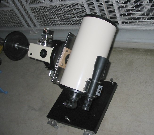
(figure 4) Telescope used to provide this data (in my "balcony"
observatory)
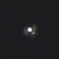
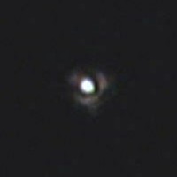
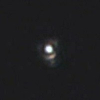
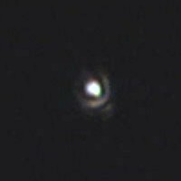
Video sequence have been recorded, 1200 images stored. The scale
is about 0.1 arcsec per pixel, focal length 10m F/D=57. The next panel shows
the best images selected out of the sequence. The exposure time is 1/100th
sec (10 ms), 20 frames per second. The field of the image is 20x20 arcsec
(Saturn globe size).
(figure 5) Images extracted from a video sequence
acquired using a Vesta Pro USB Camera, the whole AVI sequence can be retrived
here (2Mo, DivX)

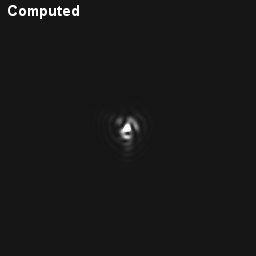
(figure 6) Computer generated image, perfect airy
disk, including 30% of central obscuration.
Now, we cannot
conclude from this sequence of video captured images, because the seeing makes
them changing at a really fast rate. Let's use our shack Hartmann
device.
When
installed, the spot pattern was recorded (single image - figure7). You may
notice less dots than the F/3.7 configuration, because the size of the pupil
is proportional to the instrument F/D ratio. If a larger pupil is required,
the 10mm focal length collimator has to be changed to 25mm. Anyway, this spot
pattern can be used.
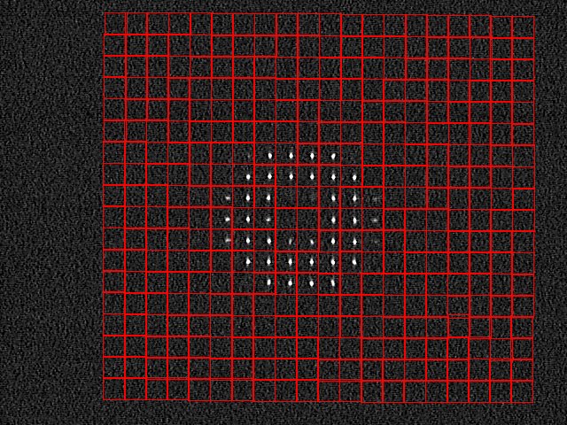
(figure 7) The red square shows the field of view of each microlense,
ie 34 arc sec in this case, this is very important to know which reference
spot matches to the measured one.
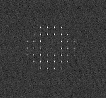
(figure 8) Single frame shack hartmann image extrracted
from 200 frames video sequence

(figure 9) 200 images stacked (canceling out the turbulence)
By stacking
up to 200 images, the turbulence effect has been canceled out, allowing us
to know the telescope optical performance, as if it would be measured in Lab.
PRISM has a
feature to reduce the data from Shack Hartmann spot pattern, which gives directly
the Point Spread Function (PSF) by computation (figure 10).
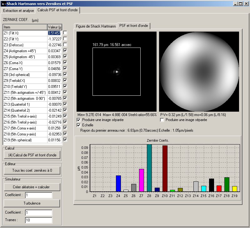
(figure 10) Data reduction software Panel
The PSF (Point
Spred Function) is not perfect (;-) it does not surprise me, because nothing
is perfect in this world :-).
The dominating aberrations are Z8,Z10 and Z7. Z7 is a little bit of coma,
that makes sense because collimating a telescope is not easy. Z8 is spherical
aberration, that also makes sense because the Matsukov is designed to have
the best correction for a given focus, or given distance between the secondary
mirror and the primary mirror. Since the main mirror is moved to focus the
system, by moving it, it adds a given value of spherical aberration The Z10
term, is related to Y trefoild, which clearly indicates that something stressed
the optics (more likely the main mirror, like optomechanical stress). Also,
the explanation could be that the telescope tube was at 22°C only 2 hours
before the measurement that took place at 1°C, may be, it missed some
more time to reach thermal equilibrium (?). I'll check it out again. Anyway
this is not so bad !
 -
- -
- 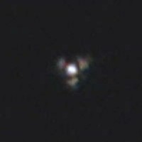
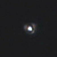
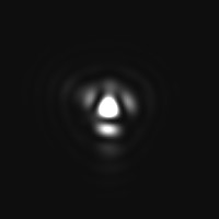
(figure 11 -12) Center : computed star shape (PSF) -
Right and left the actual PSF image from the video sequence (not a the same
time, say the most approaching), the webcam and the shack hartmann orientation
is not the same as well as the image scale.
(figure 13) Same scale as the previous left image, perfect
PSF (not including central obscuration)
The same data
reduction procedure was applied to a different shack hartmann video sequence,
I got the same computed PSF, indicating that the system is stable, and I kept
the defocus Z3 figure, by not forcing it to zero as I did usually. The figure
13a has been computed, which is very realistic compared to the actual star
video sequence.

(figure 13a)
Computed PSF + defocus
If the same
procedure is applied to a single image from the video sequence, one could
retrieve the computed PSF of a star distorted by the turbulence
-  -
-
(figure 14-15-19) Single frame shack hartmann image(Left),
Middle : the reconstructed computed PSF, Right : the most approaching image
from the video sequence recorded few minutes before.
We have
demonstrated that this apparatus is working perfectly, in agreement with video
sequence recorded by a webcam just few minutes apart. This is nice, because
now telescope optics can be characterized accurately and without no error
by this setup. Star Knife edge testing (Star Foucault test) is an interesting
test, but enable to give accurate and figures (at all) when used with real
stars.
For large
telescope (>400mm), direct imaging (as we did using the two barlows) can
not provide any valid results because the image is too much affected by turbulence,
whereas Shack Hartmann is still able to provide accurate measurments.
Here
: the link to a powerpoint presentation held during the
"2003 Aude Seminaire" (2.5Mo in French language)
See also this
link related to turbulence
References
Some papers that
helped me a lot to achieve this project...
By Cyril Cavadore
(December 2003), Back to Home Page