|
HF
Propagation tutorial
by
Bob Brown, NM7M, Ph.D. from U.C.Berkeley
Propagation
modes and DXing (VI)
Having
spent some time with the ionosphere, now we have to be more
practical, speaking of propagation modes and the things that can go
wrong when DXing. But
modes are the first order of business. In that regard, everyone
knows about HF hops from the various regions - in the range of
1,500-1,750 km from the E-region and about 3,000-3,500 km from the
F-region. Of course, it depends on frequency and the radiation angle at which signals are
launched.
The
electron distribution, having greater density at the higher
altitudes, always refracts signals downward. That may seem a bit strange but that is the case; rays which
are ascending are bent back toward the earth and the same is true of
rays which are going down. The
rate of bending is greater at the higher altitudes, when rays are
close to the greatest concentration of electrons, but it is always
AWAY from the region of higher ionization. And as I indicated earlier, how far rays proceed in the
ionosphere depends on the effective vertical frequency (EVF) when
they were launched, just like the baseball. Remember?
Let's
take the case of some rays where the EVF is very close to the
critical frequency at the peak of the F-layer. In the figure at
right, Ray A is one where the EVF is less that
foF2 and it is bent back toward ground while Ray B is one where the
EVF is greater than foF2 and it penetrates the F-peak and goes on to
Infinity.
But
notice that both rays A and B are bent or refracted AWAY from the
region where the ionization is the greatest, the F-layer peak.
That's a general feature of refraction in the upper range of the HF
spectrum. Now one other thing; it seems rays can be reversed in
electromagnetic theory so Ray B could be the path for galactic radio
noise which penetrates the F-region below. OK?
Now
we come to Ray C, one where the EVF is very, very close to the
critical frequency of the F-layer. That type of ray, moving almost parallel to the earth's
surface is called a Pedersen Ray. Those rays can give very long hops
but they are essentially unstable in the sense that any little
increase or decrease in the electron density and they diverge, going
back to ground like Ray A or off through the F-peak to Infinity like
Ray B.
Just
in case you missed the idea, Pedersen Rays at the peak of the
F-region involve the upper portion of the HF spectrum as the oblique
path must reach those altitudes; that is not possible for the bottom
of the HF spectrum (3 MHz) as even vertical rays can't penetrate
that far up in the ionosphere as foF2 is just too high.
But
that is not to say that Pedersen Rays are impossible at the bottom
of the HF spectrum; it's just that type of refraction takes place
down around the E-region where the electron density levels off for a
short range of altitude. So let's look at some ray paths there, for 80
and 160 meter signals with EVF close to the value of foE, especially at
night as shown at left.
Ray
path A corresponds to a E-hop where EVF < foE and covers only a
short distance to a receiver. But
Ray B is one where the signal has an EVF that's very, very close to
foE. But it penetrates the E-layer and ascends into the F-region;
however, its EVF is still too low to reach the higher portions of
the F-region and so it is refracted back down.
If the down-going angle of the ray has not been affected, it
will continue for a distance along the level of the E-region and
then be returned to ground. In
a sense, the path resembles that followed by a Pedersen Ray but
there is that short excursion into the F-region making it an E-F
path.
Whether
at the level of the E-region or the F-peak, paths which have
Pedersen-like refraction cover greater distances than the simple
E-or F-hops. As such,
they would contribute to paths with few hops and stronger signals;
however, as noted earlier, they may be unstable and only have brief
existences. With the
varied paths that amateurs use, such situations are not readily
identified; however, for fixed paths in commercial use, it is a
different story. In
that regard, it is pointed out in Davies' book that HF Pedersen rays
tend occur around local noon on fixed paths across the North
Atlantic, when the density gradients along the path are at a
minimum.
So
the above examples cover the simple, single hops that can occur,
from short E-hops to long E-F hops, then F-hops and even long
Pedersen hops. After that, we get into multiple hops; those are more complicated,
of course, but there is some simplicity in the second and third hops in
that reflections involve equal angles of incidence and reflection
from a surface. But even then, there is the odd chance of complexity if the surface is
not flat or not smooth. The former would, in effect, change the next launching angle of a ray,
adding or subtracting the tilt of the surface to its original angle relative to the horizontal direction.
As
for rough surfaces, they can give a diffuse reflection and that
serves to reduce the power carried forward in the original direction.
At surface reflections, there can be some signal loss,
depending on the signal polarization, surface material and the
frequency.
As you know,
we distinguish between horizontally and vertically polarized waves,
meaning the electric field of the wave is either parallel to the
earth's surface or perpendicular to it, as for radiation from a
horizontal dipole or a vertical antenna.
While
there may be signal loss (in dB) on reflection, the process is
discussed first in terms of reflection coefficients, meaning the
amplitude of the reflected wave compared to the incident wave. The
graphic at right illustrates the case for good ground material and 14
MHz signals; clearly, the small reflection coefficient for vertical
polarization around 25 degrees means there would be a large signal
loss for waves incident at that radiation angle. But horizontal polarization is much better in that regard and
is the reason why most DXers prefer horizontally polarized antennas.
Of
course, once signals leave an antenna, their progress is part of the
discussion of propagation. Everyone
knows that salt water is the best reflecting surface for RF and
fortunately 78% of the earth is covered by oceans. That really helps
DXing. But a significant fraction of ground (and amateur population)
lies in the northern hemisphere and the rest of the earth involves
ice and snow in the polar caps so the distribution of surface
material shown below is of some interest to the propagation of
signals.
We'll
do more with reflection loss later on but for the moment, it is
important to know it is there and extracts signal strength with
every bounce. But there is one more point to bear in mind; the angle
of reflection can be as important as the polarization, the surface or
frequency. Thus, losses off of water at low angles are about 1 dB, about
3 dB off of the various forms of ground and in excess of 6 dB off of
snow/ice. The situation gets progressively worse at higher radiation
angles so low radiation angles should be the order of the day. But you
knew that, just because the hops are longer at low angles.
 |
|
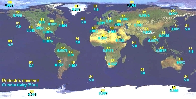
The
reflection power of the earth varies from excellent to
extremely poor depending on whether you are over salt
water (dielectric constant k=81, conductivity G=5
S/m), pastoral with medium hills and forestation (k=13,
G= 0.006 S/m) or cities with building and heavy
industries (k=3, G= 0.001 S/m). A poor ground affects
also performances of vertically polarized antennas due
to the Pseudo-Brewster Angle (PBA), a situation
similar to the one we experiment when the sun is low
and its light reflects from the water's surface as
glare, obscuring the underwater view. The reflection
coefficient can exceed 90% at 15° of elevation (21
MHz). |
|
Finally,
it should be noted that we've pretty well assumed the ionosphere to
be concentric with the spherical earth. That is a simplification, of course, and we have to expect
tilts in the ionosphere and those will have effects on waves
returned from the higher altitudes. For one thing, a tilt ALONG the path will change the angle of
return to the ground; for another, a tilt ACROSS the direction of a
path will affect the polarization in the sense that what was a
horizontally polarized wave may now have a vertical component to it.
So the next ground reflection becomes a bit more complicated,
the signal loss now depends on how the two polarizations are
reflected. And then there are phase changes on reflection. But nobody
said radio was simple, did they?
Let's
go on with multiple hops, putting in more of the details. One matter
of interest is the radiation angle throughout a path. Thus, one
might pick one angle, say at the peak of the antenna radiation
pattern, and try to follow it along a path. But while the Laws of Optics apply, with angles equal for
incidence and reflection from a surface, the angle may change due to
a tilt of the ionosphere on one hop or change of inclination or
slope of ground at a reflection point.
So
there could be some variability in the radiation angle. And, of course,
the height of the ionosphere is not constant along a path, changing if
the path goes from being in sunlight to being in darkness. All
those aspects of the path serve to change the distance per hop or,
for that matter, how close the path for a given radiation angle
comes to the target QTH.
Leaving
aside the variations which result from surface reflections and the
like, one can illustrate path structures by making various
combinations of hops. Without citing any particular type of the ionospheric
circumstances, some common paths are shown below.
 |
 |
|
At
left a propagation path close to the gray line
involving together an E- and an F-hop. At right an
F-to-F propagation involving a plasma cloud known as
an E-sporadic. Both phenomena contribute to long-path
propagation. |
|
Of
course various other combinations are possible. The modes shown above are specified as as E-F and
F-Es-F. For longer paths, the number of E- and F-hops may be larger,
depending on how the path is located relative to the terminator. As for desirability, the rule is that E-hops on a path are
where most losses occur, with ionospheric absorption on the sunlit
legs and ground losses, while F-hops in darkness have less loss,
with fewer ground reflections for a given distance from point A to
B.
The
presence of a sporadic E reflection, without any intermediate ground
reflection between reflections from the F-layer, brings up another
type of path that contributes to long-path propagation.
Here,
the idea is the same as with the Es reflection except that the
ground reflection is missing because of ionospheric tilts, shown at
left in cyan, between the two portions of the F-region.
This
figure is "Flat Earth Physics" but in reality, the
ray reflected off the first part of the F-region did bend downward
but it didn't go down far and the curved earth fell away from it so
it missed the earth and went on to the F-region again. OK?
While
the tilts shown below are exaggerated, such circumstances are found
regularly on paths going across the geomagnetic equator in the
afternoon/evening hours and give rise to long, chordal hops with
correspondingly stronger signals. But it should be noted that "tilts" really are
another way of representing the changes in the electron density
distribution along a path. Thus,
an upward tilt, one that gives a longer hop, really is the same as
the case where the electron density DECREASES along a path direction
and results in less downward refraction. That is called a negative gradient and, of course, a positive
gradient is just the opposite.
Finally,
there is another interesting variation on path structure that
results from a negative gradient along a path, ducting as displayed
above right. In that case, the situation is like the E-F hop discussed
previously but the excursions into the F-region are repeated several
times.
Again,
the representation shown at right is "Flat Earth Physics" and
involves a negative gradient, just like the chordal hop mentioned
earlier. But those long
hops are more characteristic of the upper end of the HF spectrum, 14
MHz and above, and require almost the full height of the ionosphere
for their completion. That is the case as even a reduction in electron density
along a path does not reduce refraction at the higher frequencies to
a great extent.
The
ducting shown above right is for the low end of the HF spectrum and
involves smaller vertical excursions of ray paths than the case for
chordal hops. That is
the case as refraction varies with the inverse-square of the
frequency; thus, for the same gradient or reduction in electron
density along the path, the change in the downward refraction is
much greater at the low end of the HF spectrum and less of the
ionosphere is required for the same type of effects.
Now,
having gone through a wide range of mode structures that are
possible, one can use those ideas in dealing with propagation. But,
face it, the RF from one's antenna pattern goes off into all the
possible modes, be they E-, E-F or F-hops and, depending on the
operating frequency, some of the exotic modes, like chordal hops or
chordal ducting are possible too. But the mode that gets through for your DX contact is
something of a "survivor", giving signals where the others
have died out due to absorption or have the wrong radiation angles
for the path or receiving antenna.
But
at this point, about all we're prepared to think about are the more
common modes and those would be in relatively calm, stable
conditions. In short,
we'd be looking at the indicators, SSN and the like, perhaps a map
with great-circle paths on it and pointed our beams in the right
directions. But the
"when, why and how" have yet to be discussed, to say
nothing of circumstances that are out of the ordinary.
Myself,
I consider "when, why and how" to be the "propagation
imperatives", the ideas that every DXer should have in mind
before turning on the rig in pursuit of a "New One". In short, those ideas should be "Second Nature",
the sort of thing you'd have in mind if shipwrecked on a desert
island with nothing but the makings of a ham station at your
disposal. You should be able to think of the DX QTH, have a feeling for
what could be done on a given date and think of when to get on the
band of your choice. Sometimes the answers are not to one's liking
but an answer should be forthcoming without too much
head-scratching.
So
let's see what we can do to get that right, at least for normal
conditions, and then deal with disturbances and see what they'd mean
for us. That won't be
too burdensome as once the broad outlines are established, you'll
have a propagation program to fill in the quantitative details, case
by case.
Now
we've discussed some of the general ideas behind propagation in the
HF part of the spectrum and you should have a good grasp of what it
all depends on - enough ionization overhead to refract signals
downward, keeping them in the F-region, and signals getting through
the ionization down in the D-region with enough strength to overcome
the local noise.
Case
study
With
that in mind, let's explore propagation with a practical case, say
making a contact between a central location in the USA and Togo,
West Africa in the upcoming CQ WW CW contest in late November 1998. That'd be a good test to see just how far we can go in
predicting propagation using the simple ideas developed so far. That
done, we can look at how computer programs do it and see what other
details they offer.
So
let's use Omaha, NE as our QTH in the USA; that's at 41° N, 96° W. Togo
is a bit harder so we have to go to the ARRL Operating Manual or
DXAtlas to find that it's located in the Horn of Africa, at 6° N, 1° E,
close to the Greenwich Meridian. Looking
at those coordinates, one thing is immediately clear - it's quite a
ways from Omaha to Togo, more than 90° difference in
longitude and more than 35° difference in latitude.
 |
 |
|
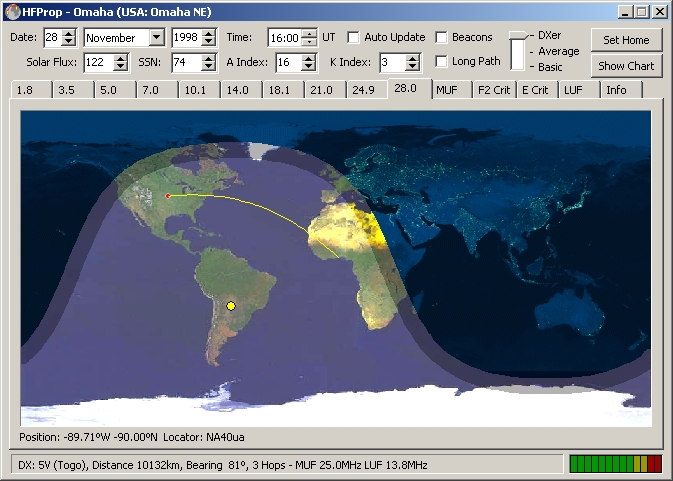
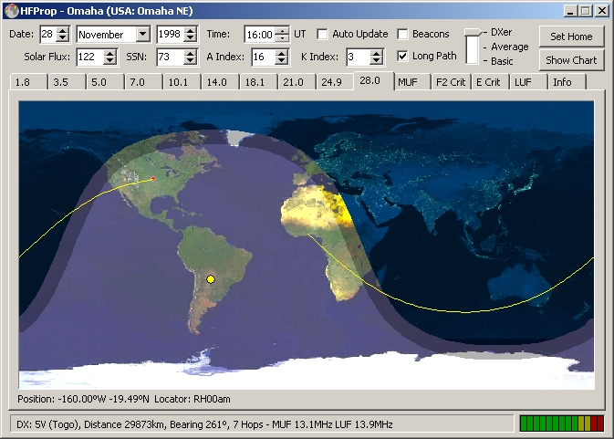
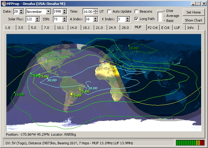
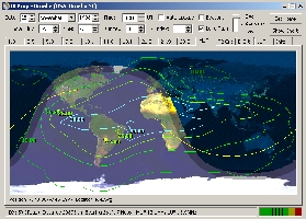
To
reach Togo (5V) by
shortwaves from Omaha (NE., USA) you have two
solutions : use the short path (10,100 km bearing
81°, 5 hops) or the long path (29,900 km, bearing
261°, about 10 hops). The direct and short path to
this central african country seems "workable"
and accessible as the 3/4th of the path runs over the
ocean that offers a high reflectivity to shortwaves.
The long path is also interesting as it runs on 5/6th
of the path over the dark side of the earth. But first
of all is there an opening to Togo on 28 MHz by 1600
UTC on this November 21, 1998 ? The solar and
geomagnetic conditions as well as the MUF and the F2
critical frequency maps will help us to answer to this
question. In the
negative we will have to work this entity at another
time and another band, maybe much lower. The answer is
given you below. map created with HFProp. |
|
Considering
that the distance around the earth is about 40,000 km, one can
conclude immediately that the distance to Togo from Omaha is better
than 10,000 km, a quarter the way around the world. That's confirmed
by going to the azimuthal equidistant map for Central USA in the
ARRL Operating Manual or any logging program showing the world map
(e.g. DX4Win); Togo is half way to the antipodal circle, making it quite
a haul. But it's not all that hard if you're on the right band at the
right time.
Now
we're talking about late November so we can take the
effective sunspot number SSN as around 80, judging by recent reports
from NOAA. The chances
of making a contact on the higher bands are pretty good when you
consider that Togo is at a low latitude, where the the electron
distribution of the F-region is quite robust. So we only have to worry about launching the high band RF
from Omaha.
As
a first approximation, let's think of trying for a contact on 28 MHz.
For that, ionization and the MUF are the important things and tell us that the
contact should be tried during the time the path is well illuminated.
So with a longitude difference of about 97 degrees, we'd like to have the sun
at least midway between the two QTHs, say at about 47° W of longitude.
With the sun advancing westward at 15° of longitude per hour, that means
the time should be about 3 hours after 1200 UTC or 1500 UTC.
But
remember Togo is at a low latitude so the critical frequency of the
F-region there is less of a problem than at Omaha. That being the case, it would be better to choose a later
hour, one when the sun is closer to the longitude of Omaha, raising
the critical frequency near there. But the time should not be so late as to have the sun set
anywhere on the path. That means we have to look into the sunrise/sunset tables in
the ARRL Operating Manual or any astronomical calendar, paper or
program, and see when the sun would set at Togo.
 |
 |
|
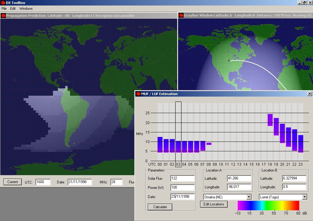
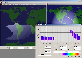
At
left, the MUF iso-contour map calculated with HFProp
shows some "islands" up to 30 MHz between Equator and
Kenya, at first sight good to reach Togo; the short path looks open.
But at right, the F2-critical map shows many areas where
the critical frequency is much lower (6-8 MHz). Other maps,
especially the MUF, the propagation map, SNR and reliability
charts will confirm that in fact all bands from 20 to 10m are open
to Togo in this evening (1800-0100 UTC) with signal between S6
and S7. Unfortunately in the afternoon signals are not
higher than S3. |
|
In
that regard, the Operating Manual gives SR/SS data for November 21
and we can use that as an approximation, taking the ground sunset at
Togo as 1736 UTC. That would suggest, as a first correction, that the 28 MHz band be tried
between 1530 UTC and 1730 UTC. The same would apply for 21 MHz too, knowing that less
ionization is needed for propagation on that band, so an operating
window might be better if widened to start earlier and end later,
say from 1500 UTC to 1800 UTC.
As
an aside, I should say that last idea has some generality to it, at
least for the bands where MUF are important. So from a given QTH, the
lowest bands open the earliest, the highest bands the latest, and band
closing is in reverse order. Of course, that is just the availability of the path; the
signal/noise situation still has to be looked at for the best times
of operation.
As
for the transition bands, 10 MHz to 18 MHz, absorption plays a role
there and good sense indicates the effect can be minimized by
avoiding times when the path is well illuminated, with the sun
around its midpoint. In addition, we know that ionization lingers after sunset,
thanks to the role of the geomagnetic field and the slow
recombination rate of electrons and positive ions up there in the
F-region. As a result, propagation on those bands would be supported
around sunset and on into the evening hours.
In
addition, the rising sun on the path near Omaha would open up
propagation, at least until absorption became too great. That
being the case, we can expect the bands to open shortly
after the sunrise at Omaha, roughly 1350 UTC according to the
Operating Manual. And with sunset around 1730 UTC at Togo, another
two or three hours could be added to the operating time.
Things
are shaping up, at least for the bands where F-region ionization and
D-region absorption are important. That would give a starting point as sunrise at Omaha, about
1400 UTC, and a closing time of about 2030 UTC for the transition
bands. The higher bands would start later, of course, and end sooner,
the general principle mentioned earlier.
The
lower bands, 160 meters - 40 meters, where D-region absorption
dominates, would be open from sunset at Omaha til sunrise at Togo.
Going to the Operating Manual, we find low-band operations could
start at Omaha around 2300 UTC and end around 0545 UTC.
 |
 |
|
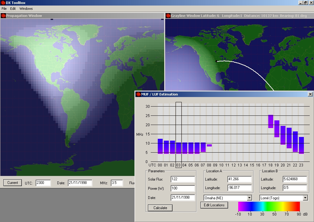
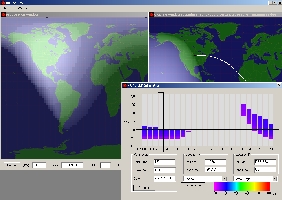
At
left the MUF calculated by DX
Toolbox over Togo does not extend over 24 MHz
around 1800 UTC and goes down to 10 MHz during the
night. In fact from Omaha, at 1600 UTC the only
opening on 10m is toward South America. To reach
Togo in good conditions we must go down close to 20m and work late
in the evening (2100-2300 UTC and even early in the
morning on the low bands as shown at right). The signal
are predicted weak,
thus to work preferably in CW or in SSB with 1 kW in a
directional array. You lost
your time if you try to work 5V at another time. Other
charts will confirm these conditions. |
|
But
there is the question of noise, man-made or atmospheric in origin,
to compete with signals. Here, experience shows that man- made noise
is less as the hour goes past the end of the working day. And
atmospheric noise, say at Togo, would be the lowest at times close
to dawn. So low-band operation probably would be more productive in
the later hours of the operating window. But in view of the high level of ionospheric absorption and
distance involved, it could be much more difficult to make a contact
on the lower bands than the higher ones. In addition, antennas and power
play a greater role in that part of the spectrum. Those
resources are developed over time by DXers and related to their
operating experience in that part of the amateur spectrum. Put another way, DXing on the lower bands, 80 and 160 meters,
is tough and not always rewarding for casual operators.
Now,
to add a realistic twist to this discussion, let me say that I
worked 5V7A on 20 in CW at 2312 UTC on November 29, 1997. If you look into it,
you will see that was over five hours AFTER ground level sunset at Togo!
(See? Ionization does linger on in the dark, especially at low latitudes!)
I would hope you could do the same this year. At least, the above example shows how you can
"sharpshoot" for a New One, even with only primitive tools
at one's disposal. Give it a try. OK?
 |
 |
|
At
left for a S/N ratio reliability (SNR) of 38 dB in CW
and a required reliability of 90% at the specified date
(Novembre 1997) and with a SSN of 40, VOACAP
predicts a S/N ratio of 40 dB in Togo at the time of
Bob's QSO with 5V7A at 2312 UTC. At right taking into
account the date and URSI/88 Coefficients, ICEPAC
predicts for the opposite circuit a signal power in
Omaha of -117 dBW, or close to S7. A QSO can be sched
at that time with good signals on both sides. Bob selected the best time; according
forecasts, signals were the strongest on 20m between
2100-2300 UTC as predicted DX Toolbox as well. Note
that both circuits (K-5V or 5V-K) are quasi reciprocal
with very light differences in the signal strength,
MUF and FOT. |
|
Now
I didn't work out all the aspects of contest propagation for the
5V7A group; you'll see what their own propagation guru came up with
but I'm sure it was based on the principles I outlined above. I have
done that sort of thing before, for the recent 8Q7AA and 3B7RF
DXpeditions. In that sort of circumstance, the idea is to forecast so they
can "Work the World". So every time interval has to be looked and in every
direction to find the best way for them to operate in the contest.
The
first one for the 8Q7AA group went very well, operations going
essentially as predicted. But
the second one for 3B7RF got into a bit of trouble; that was
interesting in itself as it will lead us into the matter of
ionospheric disturbances of geophysical origin. Leaving that to
later, let's go beyond slow, mechanical methods, how "The
Ancients" handled the propagation problem, and look at how it's
done by computers.
As
you know, they do everything practically at the speed of light. But
how well do they do it? That's a good question. As a
matter of fact, given what you know now, you might wonder if they
just do the old-fashioned calculations faster and not add much to
the problem. So we'll go with that for a while, looking at how computers
handle these questions and then look at a few new ideas.
Reference
Notes
If
DX contesting is the sort of thing that interests you, let me say
that the 5V7A crew were kind enough to provide me with their '96 and
'97 contest logs for analysis. I was more interested in them for the aspects of 160 meter
propagation but you might look at my article in the March/April '98
issue of The DX Magazine.
It also shows how demographics overpowers propagation.
Next
chapter
Propagation prediction programs
|