All about Transmission lines

As a part of voltages and currents flowing in the line are reflected, usually between 0.5-5%, due to phase shifts, these components see their respective amplitudes and phase vary in respect to their position on the line.

If we plot the resultant voltage and current in a graph against their respective position along the line, we observe curves. If the load perfectly matches the line impedance, the graph shows that the voltage and the current are the same everywhere along the line. If the load is less than the line impedance, we observe variations in amplitude due to the mismatch between the load and the line; these wave-like curves are called standing waves. If the load is greater than the line impedance we observe the same curves, excepted that the case is inverted : the current curve becomes the voltage curve and vice versa. This is of course a mathematic representation because no wave are really standing, at rest, as observed Einstein one century ago.

Closely analyzed this graph has several characteristics. First, at a position 180° or 1/2λ from the load, both voltage and current have the same value they do at the load. At a position 90° or 1/4λ from the load the voltage and current and inverted : when the voltage is high, the current is low at the load and vice versa. At last at 270° or 3/4λ from the load the 90° point is duplicated. In fact if we continue the graph toward the source we will observe than every point odd multiple of 90° or quarter wavelength duplicate. In the same way the voltage and current are the same every point multiple of180° or one-half wavelength as they are at the load.

The ratio of the maximum voltage along the line to the minimum of voltage is called the voltage standing-wave ratio, VSWR for short. We can also use the ratio of current in the same way as the VSWR. In most magazine and in the common language we simply speak in terms of SWR ratio and this is this way that are labelled most SWR and power meters.

So using a simple external SWR-meter we can estimate with a good accuracy the line performance, the emitting power, the percentage of reflected power, and therefore its SWR.

If SWR represent the ratio of voltage or current, it gives also the matching quality between the characteristic impedance of the feed line and the (resistive) load. If the load contains no reactance, the SWR is equals to the ratio between the load resistance R and the characteristic impedance Z_o of the line:

As the smallest quantity is always in the denominator, the SWR is always greater than 1:1.

In the standing wave graph displayed previously, we observed that for a line which length is 180° (1/2λ) or a multiple of 180°, the voltage and current have the same value as at the load. That means that the source of energy "sees" a resistance equals to the actual load resistance at these line lengths. In other words the impedance has both resistive and reactive components. When the current stays behind the voltage the reactance is inductive; when it leads the voltage the reactance is capacitive. Practically when the R < Z_o, the reactance is inductive in the first 90° or quarter wavelength going from the load to the generator, is capacitive in the second 90°, inductive in the third 90°, and so on every 90°. If R > Z_o, the voltage and current are interchanged; the reactance becomes capacitive in the first 90°, and so on.

The amplitude and phase angle of the imput impedance is also determined by the SWR, the line length and its characteristic impedance. When the SWR is small (say below 3:1) the input impedance is mainly resistive; if the SWR is high, the input impedance is mainly reactive. We usually represent these impedances by a equivalent series circuits constitued of resistance and coil or capactors as displayed below, where Rs is the resistive component and Xs th reactive component. In formulae the "s" are often omitted and the series equivalent impedance is note as Z=R±jX. The "j" factor is in fact an operator indicating that the values for R and X cannot be added directly, but that the vectorial addition (like in the resolution of vectorial triangles) must be used if the overall impedance is to be calculated. By convention a plus sign is assigned to j when the reactance is inductive (R+jX), and a minus sign is assigned to j when the reactance is capactive (R-jX).

At last up to now we only considered pure resistive load. In the field this is practically the case as the antenna connected to the end of the feed line is resonant and thus resistive in nature. However if the antenna is well tuned to work on a specific frequency, at a few hundreds kHz away from the centre of the band for which the antenna is cut or on other bands it can display some amount of reactance along with resistance. In other words your SWR will increase. The direct effect of this reactance in the load will be to shift the phase of current according the voltage both in the load and the one reflected. If the reactance is inductive the phase (point of maximum voltage and minimum current) is shifted toward the load and vice versa if the reactance is capacitive.

In the field, as soon as the input impedance is not purely resistive it displays some resistance or reactance. These properties can be modelized by using electrical circuits either in series or in parallel as displayed above.

In 1939, the US magazine Electronics published original graphs in wich the rectangular coordinate system was replaced with curved coordinate lines and fill in with excentric circles of all sizes. These graphs had to help amateurs in calculating resistance and reactance of circuits like transmissions line or antennas. Its inventor was Phillip H.Smith, from Analog Instruments in New Jersey.

In fact a Smith graph as this representation is now called, is nothing else than a coordinates system, curved rather than rectangular, showing only one axis, the resistance axis, which is the only straight line cutting the graph in two parts. It includes also resistance circles that are centered on the resistance axis; they are thus tangent to the outer circle of resistance. Each circle displays a value of resistance, indicated at the point where the circle crosses the resistance axis. All points along any one circle have the same resistance value.

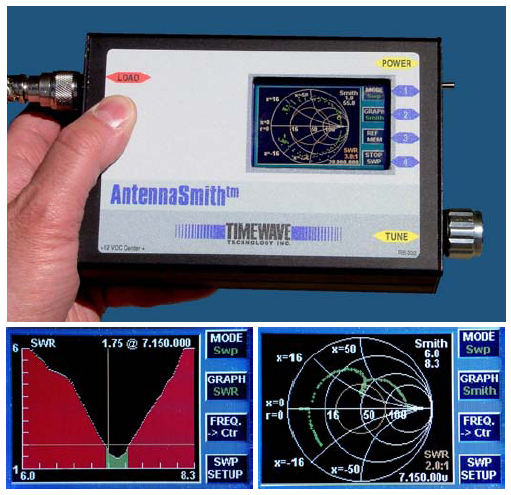
This chart replaces all computers and like the old slide rule it can help you in calculating properties of transmission lines (resistance, reactance, capacitive).

Associated to wavelength scales, standing wave scale, reflection-coefficient-voltage scale, transmission losses and losses in dB scales, the Smith graph becomes a complete manual calculator able to calculate SWR, reflected power or antenna impedance.

We cannot discuss any longer on this page about such graphs as the subject, without being complex requires many examples to be well understood, what cannot be summarized in some paragraphs. I suggest you to refer to the ARRL Antenna Book for more detail about Smith charts.

At last, since 2005, Timewave sells an antenna impedance analyzer model "TZ-900 AntennaSmith" ($999.95) displayed at left. It is a small box operating between 0.5 and 60 MHz able to simulate on its small TFT screen SWR graphs and Smith charts in full color.

Up to now we have considered perfect transmission lines without loss. However losses are inherent to the use of lines due to several factors. First there is the conductor resistance that lets flow more or less electrons; then there are dielectric properties of the conductor insulating that consumes some power; and at last a small amount of energy migrates to the outer surface of the conductor and escapes in radiating some power.

These losses modify slightly both the line characteristic impedance and input impedance because of the changing of the line resistance, but they are usually not sufficient to prevent you emitting. In fact, losses of power are due to three main factors : first the length of the transmission line that attenuates slightly signals of a few decibels, then there are losses due to the wire characteristics called the loss per unit length, and at last the ones due to a high SWR. The effect is more appreciable with long lines (up to 50 or 100 m), where losses can exceed 10 dB on UHF or reach 5 times that value depending on the cable design as show in the table below.

Coax Cable Signal Loss (Attenuation) in dB per 10 m
Loss	RG-58	RG-8X	RG-213	RG-6	RG-11	RF-9913
1 MHz	0.1dB	0.1dB	0.1dB	0.1dB	0.1dB	0.1dB
10 MHz	0.5dB	0.3dB	0.2dB	0.2dB	0.1dB	0.1dB
50 MHz	1.1dB	0.8dB	0.5dB	0.5dB	0.3dB	0.3dB
100 MHz	1.6dB	1.2dB	0.7dB	0.7dB	0.5dB	0.5dB
200 MHz	2.4dB	1.8dB	1.1dB	0.9dB	0.8dB	0.6dB
400 MHz	3.7dB	2.6dB	1.6dB	1.4dB	1.2dB	0.9dB
700 MHz	5.6dB	3.7dB	2.2dB	1.9dB	1.6dB	1.2dB
900 MHz	6.7dB	4.2dB	2.6dB	2.0dB	1.8dB	1.4dB
1 GHz	7.2dB	4.5dB	2.8dB	2.0dB	1.9dB	1.5dB
Ω	50	50	50	75	75	50
Coaxial losses shown above are for 10 m (3 ft) lengths. Loss is a length multiplier, so a 20 m length would have twice the loss shown above and a 5 m length would have half that loss. This multiplier factor means that you should keep cable installation lengths between your RTX and antennas as short as practical !

Power lost in the transmission line varies as a logarithmic function of the length, hence is expression in terms of decibels per unit length, which is also a logarithmic measure.

Line loss, conductor loss and dielectric loss increase with the frequency, but not linearly and not the same way. Therefore there is no formula to calculate the overall value but tables that give for each frequency and each types of line the relationship between these three parameters.

At last, when SWR increases, both current and voltage become larger what increases power losses and thus attenuation. A SWR 2:1 causes a power lost of about 0.5 dB whereas an SWR 4:1 produces already a 4 dB loss. But it is important to note that SWR curves like the ones displayed below represent values that exists at the load, practically at the antenna terminating a feed line and not at all the SWR at transmitter; in the worst case, in presence of high SWR at the load (say over 10:1), the difference reach a 2- to 10-factor ! However, it is good to know that when the line loss is high with perfect matching, the additional loss causes by the SWR tends to be constant regardless of the matched line loss.

As we explained in the page dealing with SWR, many amateurs do not use an external SWR-meter and trust the built-in meter of their transmitter. However this reading will always display a lower value than the real SWR existing at the antenna, because at the transmitter the attenuation is not taken into account yet. Of course it is not always convenient to measure SWR directly at the antenna when it is erected 15 meter high, Hi!, but a good value is to pick up this measure along the coaxial, between the transmitter (or the linear amplifier) and the antenna.

Until now we have discussed of voltage and current on lines, never in terms on power. In fact we learnt during the preparation of the radioelectricity exam that the power is proportional to the square of either the voltage or current (P=RI² or P=E²/R). Remind that the ratio of the reflected voltage or current, the reflection coefficient r at the load is :

Let's take the case of 100 W of power put in a matched line with a SWR 4:1. The reflection coefficient ρ = 60%. Thus the reflected power is 0.6² = 0.36 times the incident power, or 36 W. That amount of power comes back at the input terminal, leaving only 64 W of power for the source. To put 100 W in the load, the coupling to the source must be increased so that the incident power minus the reflected power equals 100 . Since the load absorbs 64 W, the incident power must be 100/0.64 = 156 W.

At left, the increase of current or voltage according the SWR. The line voltage and current are directly proportional to the square root of the SWR. At right, what happened to PL connectors sustaining too high power and SWR. The connector at foreground was placed outdoor in ambiant moisture. It sustained a power of 850 W with an SWR over 4:1. More than 75% of the power was loss in the transmission line as heat. Mixed to the moisture, the connector burnt to smoke. The other ones, placed indoor were also damaged near the central pin. So a good advice : these PL-259 being not weatherproof, protect them well if you have to leave them outdoor and never use your transceiver with a too high SWR (say over 3:1) at risk to get serious troubles, including fire if your connectors touch a stock of paper, plastic or chemical products. In presence of high SWR and high power you might also experiment arcing when touching these PLs and be injured. These connectors are very appreciated and performing but use them safely. Take care !

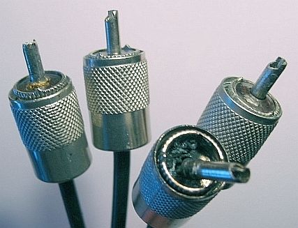
But working this way has one major drawback, the increasing of voltage and current in the line. Indeed, in applying the formula for the power, I=√(P/R) and E=√(PR), for a line which characteristic impedance is 50 Ω, if 100 W produces 1.41 A and 61 V, with 156 W in input we get 1.77 A and 88 V on the line. If we take into account line losses of say 3 dB, only half that power will reach the antenna and the input power must thus be still increased to about 300 W with still more current and voltage to get 100 W at the antenna. Your coaxial and connectors might not support this current and burn to smoke !

This way of "tuning" your antenna system (line and load coupled) is not professional and far to meet skills of radio amateurs. In fact as shows the graph displays above, beside the search for the lowest SWR as possible, there are curves to respect, showing the maximum possible value of current or voltage that can exist along a line with a given SWR. Pushing your input power too high with a high SWR you risk to request 5 times more input voltage and current and no more operate in a safely way. And this is still more important using an amplifier.

The current can indeed increases much on the line and burn your coaxial plug or any object nearby it, and all the more if is not protected again moisture. Do not forget also that the RG-58C coaxial sustains a maximum of 1900 V (rms) but only 550 W PEP up to 30 MHz (105 W at 400 MHz). If you even hear some arcing while working on the air or shortcuts on your plug, switch immediately your TX off and your possible amplifier and check your transmission line...