|
Software review
|
|
|
Close
up on the System group. |
VOACAP
propagation analysis and prediction program (III)
System group
This
is a set of six fields which importance appears often at a second reading if you
are not used to VOACAP and haven't taken the time to read additional
documentation to master the program.
The
System group is one of the most important because its settings (of course in
addition to the others) affect the prediction accuracy and reliability,
essentially output parameters like SNR and REL.
Caricaturing, we can say that a wrong value inserted in half of these fields,
can transform your forecast in anything but a prediction that matches your real
working conditions ! So let's see each field in detail and how to adjust them.
Man-Made
Noise level
To
not confuse with natural noise (QRN). This is the expected QRM at the receive
location expressed in dBW.Hz (or dBW, decibels below 1W).
This value is calculated by reference to a noise of 1 Hz bandwidth at 3 MHz. The
default value is -145 dBW or S2. Not all applications use the same threshold.
Here are for example the receive noise levels set in VOACAP vs. WinCAP Wizard :
|
Area |
VOACAP |
WinCAP |
|
Industrial |
-140.4
dBW |
-125
dBW |
|
Residential |
-144.7
dBW |
-136
dBW |
|
Rural |
-150.0
dBW |
-148
dBW |
|
Remote |
-163.6
dBW |
-164
dBW |
|
Default
QRM level associated to the receive location. Note that since
the release of VOACAP ten years ago, WinCAP Wizard found that it was
more realistic to increase the QRM level in the most inhabited
areas, a sign of times... Note that -125 dBW is a good S5. |
|
They
are of course theoretical values. Most of the time you even don't know what DX
station will answer to your call and thus neither in what type of area lives
your correspondent or what is his or her QRM level. The QRM can also vanish as
fast as it appeared. These approximations can however be specified during the QSO
or earlier, when you planned your activity.
On remote islands, in the country or in the bush at tens of kilometers away from
cities where the QRM strength is unreadable on the S-meter, you can easily use the lowest value of -164 dBW.
The difference between extremes (Remote-Industrial) can make the S/N ratio at receiver drop of
20 dB, or 2 S-units, a power ratio of 100
times ! If the band is not in good shape, and whatever the SSN, that means that
it could be close under these conditions. Thus better to use the appropriate
value to get here also an accurate prediction.
Required
Circuit Reliability (%), aka SNRxx
This field is
probably the most important and requests some a detailled
explanation. As we just explained, a forecast is a prediction, a probability estimation
to work in specified conditions (the "circuit"). The term "Reliability" means
"time availability". When you set the required reliability at 50%, it means that the
resulting predictions will be as stated or better during the half of
the month, or 15 days over a 30-day month. That means also that during the other 15 days,
the actual conditions may be worse. So, SNRxx characterizes
the expected signal quality that you consider as acceptable. It is maybe valid
for you and today, but tomorrow you will maybe prefer working in "Hi-Fi
conditions" as far as possible...
But
then, why to not set SNRxx to 100%, do you wonder ? Well, if you set required
reliability at, say 90% as suggest VOA engineers, then predictions will be as stated or
better during 27 days over 30. Theoretically, in average, amateur working conditions match with a
90% reliability. In the field, that means that the concerned frequency is highly reliable, like
the "BUF".
This
is however a high value mainly suited to broadcasters that use 100 kW emitters, or big
contest teams and so big DX-peditions who work in rocking-chair, Hi ! A casual amateur might satisfy with only
50%, but of course the higher the best, all the more that the advanced amateur
will probably no more work like a casual amateur. Indeed, the beginner works
often whatever propagation conditions (even in close bands !), where the Old
Timer, experimented, will only switch his or her transceiver when the
propagation will be good to excellent to avoid useless QRN and poor propagation
conditions. Thus setting SNRxx depends also on your habits and your know-how.
But in all cases it is interesting to set this parameter to 50% and 90% to see
the change on the signal strength and pwoer at the target location.
In
addition we can say from experimental trials that the reliability reaches
90% when the geomagnetic index Ap ≤ 27 and Kp index ≤ 4, so during phases of quiet sun or so.
This
entry will of course affects the calculation of the output parameter "SNRxx".
Note that VOACAP does not display iso-contour map when you request the output
parameter SNRxx. This function is only supported in ICEPAC, included in the same
package. As we will see later, ICEPAC takes also into account disturbed
conditions near polar caps.
Required S/N ratio (dB), aka SNR
This
is the second very important parameter that must be set correctly. SNR is ranging between -30 and 99
dB.Hz, a very wide power spectrum, hence all the importance to set it correctly too.
Technically speaking, take a deep breath, SNR characterizes the ratio of the hourly median signal power in the
specified bandwidth relative to the hourly median noise in a 1 Hertz bandwidth
which is necessary to achieve the type and quality of service (mode) required,
hence its name...
Say
simpler, Hi !, this is the amplitude of your signal over the noise at target location.
This signal-to-noise ratio is valid 50% of days in a month. It is set for a receiver
bandwidth of 1 Hz (for noise only) anddepends on the mode, what VOACAP engineers called
the "service" used according to the next relation :
SNR (dB) = 10 + 10 log (bandwidth in Hz)
For
example, in SSB a signal offering a 3 kHz bandwidth gives a SNR of 45 dB. A 500
Hz CW tone is close to 38 dB. A digital mode, using a larger bandwidth, will give
a still higher ratio.
VOACAP
uses a default value of 73 dB what is qualified as "Good".
Here are "milestone" values associated to the SNR :
| Service
(mode) |
Bad |
Poor |
Fair |
Good |
Excellent |
|
BCL
~10 kHz |
<
52 |
52
- 64 |
65
- 77 |
78
- 87 |
88
+ |
|
SSB
2.5 kHz |
<
49 |
49 -
63 |
62
- 74 |
75
- 84 |
85
+ |
|
CW
250 Hz |
<
40 |
40
- 47 |
48
- 54 |
55
- 61 |
62
+ |
|
SNR
value and signal quality associated to usual modes (services). A
digital mode will give a still higher ratio. Values include an
allowance of 12 dB for fades. |
|
Note
that VOACAP engineers use the word "service" instead of
"mode" that we use when we speak about CW, SSB or SSTV modulation mode for
example to not make the confusion with propagation modes (2F, 3F2, etc). To
avoid questions during this review, I will use both words together.
Although
the SNR can vary, and varies from people to people depending on the signal
quality you want to achieve for the concerned service (mode), it is recommended to use standards values, and for
example to not set a too high SNR that seldom matches common working conditions
of amateurs. We usualy state that over 75 dB in SSB, the signal quality is really very
good, typical of a regional broadcast station; many amateur satisfy with poorer
conditions close to 50 dB,
even less in crowed bands or in presence of atmospherics. As soon as your hear QRN or
QRM on your frequency (like a strong "white noise") you can already
reduce the required SNR of about 10 or 20 dB. Idem in presence of fading. Therefore more than 80 dB is
really exceptional, a quality that I would qualify of "Hi-Fi" or
"FM grade", Hi !
In
CW for example, many amateurs work in heavy QRM conditions or use a very narrow
bandwidth in cascading several DSP filters. We can set the SNR for CW as low as
24 (Poor); in SSB in poor working conditions the SNR can be set as low as 44; at
last in you listen to DX broadcast stations, the SRN can be set as low as 65. Of
course any higher value will improve your signal but it will also mean that
VOACAP will calculate a higher reliability, thus conditions more restrictive
(pessimistic) too, but also probably valid more days per month.
Associated
to the SNRxx, these both factors will amplify or decrease the "grade"
of the expected S/N ratio. Incorrectly set they will emphasize extremes, with
for consequence to false all your prediction, showing for example a wide opening
with strong S/N where the band is in reality almost close, and the opposite.
Case
study : reliability factor in VOACAP and ICEPAC
Let's
see an example showing the influence of SNR and circuit reliability (SNRxx) on
band conditions. Below are three predictions of the required circuit reliability
calculated with VOACAP and ICEPAC for a circuit between Belgium and
Arctic Bay in Far North Canada (73.03° N, 85.18° W) scheduled in
September 2000 (solar maximum) for a SSN of 122 and 100 W PEP output.
The QSO was not succeeded. Try to know why.
To
reach VY0 sky-waves pass over Iceland. Unfortunately, at that time the PCA exceeded 150 dB at 2200 UTC
near Iceland, just mid-way to Arctic Bay, as confirms DXAtlas.
This auroral oval was very active and affected thus high latitude
propagation. As it, its intensity and its effects on propagation are
not taken into account by the program, because VOACAP has no model to calculate
them and no connexion with the outside world to update its data, but other
VOACAP-based applications use near-real-time data to forecast these
disturbances. Unlike VOACAP, ICEPAC is completed with a special IONED model that
uses some functions dedicated to high latitudes of the northern hemisphere,
taking into account several events related to aurora. But here also, working
offline with median values, ICEPAC can only "see" the high latitude of
the VY0 station, and takes only into account an average auroral activity. Its
predictions are however more accurate than the ones of VOACAP as shows very well
the next example.
Minimum
takeoff angle, aka MTA
It
is the minimum takeoff angle of the main lobe of the transmit antenna expressed
in degrees. Values accepted are ranging between 0.1 and 40° of elevation, and
for simple ray hops only.
Unfortunately,
almost each word of this definition request a comment, and not the least because
the takeoff and arrival angles of your signal affect much its strength at target
location. Under VOACAP two parameters are badly defined and are subject to
interpretation too : the elevation angle considered as fixed, and the angles of
arrival that are very inadequate.
First
let's see the elevation angle. We explained in the first page that VOACAP
inherited some settings from IONCAP, and among them there is the takeoff angle,
or rather its updated value. I explain. IONCAP used by default a MTA of 3°. But
for their broadcasting activities, VOA engineers designed special variable beam
arrays showing considerable gain below 3°. Therefore developers changed the
default from 3° to 0.1° of elevation. In theory this is an advantage because
using so low angle VOACAP will predict less transmission losses with a shorter
path and stronger signal at target location. But is it really realistic ?
In
VOACAP the default MTA is set to 0.1° of elevation. What does it mean ? By
definition only an isotropic antenna displays
in free space the same constant gain of 0 dBi between 0-90° of elevation
as shows the hyperlinked graph. But in the field, even an isotropic antenna will
be affected by the ground and will more than probably display at 0.1° of
elevation a gain almost infinite over a ground plane. This is for this reason
that in WinCAP the elevation is set by defaut to a more realistic value of 3.0°, which is
already an excellent minimum takeoff angle.
 |
 |
|
Radiation
pattern of a 3-element Yagi placed 7m high for the 20m band
calculated with HFANT. The maximum gain is 11 dBi (8.9 dBd) at
29° of elevation and drops to -30 dB, thus to a power ratio 1000 times lower at
ground level. For VOACAP, in all cases where your maximum gain is
at angles above 3° of elevation, you must set the minimum takeoff
angle at 3° only. |
|
What
is the right elevation to set in VOACAP ? According George Lane, if your antenna
main lobe is over 3°, even at 10 or 20° of elevation you must set the minimum
takeoff angle at 3° of elevation only, not more. If you enter the value for
your antenna maximum gain, for example 29° fo elevation as display above,
VOACAP will reduce the MUF with all consequences on your hops and signal
strength.
For
example, as show well the two next predictions established for a circuit between Argentina
and Belgium in September 2004 (SSN = 27), a MTA of 30° of elevation
reduces your chance to work a DX station to practically nothing; the takeoff
angle is too high and your signal enters the F2-layer under a too steep angle.
The result ? Your signal falls much closer than expected and a small amount of
your input power reaches the DX. Your signal strength at target
location is only... -233 dBW on 20m, you are in the background hash ! On the same
circuit, another antenna showing a MTA of 5° only will show a signal
strength of -133 dBW or S4. Knowing that you reduce your power by 50% each time
you lost 3 dB, working at 30° of elevation you must expect a signal lost of 41
dB, 4 S-units or a power ratio over 10000 times lower !
 |
 |
|
VOACAP
prediction for a low (3°) and high (30°) minimum takeoff angle for a
circuit between Hawaii and Belgium in September 2004 (SSN =
27). Where the 20-m band is open in the first case, if you work
with a takeoff angle over 30° of elevation, your chance to work
DX stations in good conditions are almost null, especially during
periods of low solar activities. You signal will be near the
background hash and your correspondent will probably lost your
signal from time to time as if the band was close. |
|
One
must not be clever to understand what that means for you as well as for VOACAP :
the band is close, the estimated "MUF" is two or three bands lower
than expected and only a kW-class amplifier might help you to work this DX in
these very bad conditions.
At
last, there is the problem of the angles of arrival. VOACAP doesn't work with
multiple ray hops. One can thus consider that it is almost blind to predict the
adequate pattern of arrival angles at target location. Why ? Without PropLab Pro
of a similar ray tracing application, you don't know either at what angle sky
waves will reach the distant station (all depend on the status of ionospheric layers, your
signal power, takeoff angle, multipath, delay, azimuthal spread, among other variables),
what will be the absorption level and thus the S/N ratio at receive location, and
you ignore what mode are used (ordinary, N, M, etc). These are as many parameters that are
bypassed in VOACAP and that will false the prediction to some extents. But this
is not all.
Add
to this long list that without the Skyloc interferometer system (aka Andrew
angle of arrival system) you cannot measure angles of arrival, phase difference
and amplitudes of sky waves. For VOACAP, and many other models using single ray
hops, the propagation of sky waves is quite simple, using ordinary modes, and
angles are fixed in both elevation and azimuth. But reality is far different !
In the field, using the Skyloc system we can show that in a 5-minute interval
strongest signals can spread up to 30° of elevation and 3° in azimuth although
VOACAP predicts a clustering or rays within a few degrees.
Multipath
Power Tolerance (dB)
It
is expressed in percent. Its meaning is simpler that what it seems to
state... but here also take a deep breath, Hi ! With words
borrowed to physicists, it is the maximum difference in delayed signal power
between sky-wave modes to permit satisfactory system performance in the presence of multiple signals.
Oops ! It concerns in fact effects of multiple sky-waves pathes using various
modes on the strength of your signal. This probability gives you an estimation
whether or not multiples sky-wave modes exist within the specified power tolerance and outside the time delay
tolerance (see below). A very large tolerance spreads your signal in many pathes
and affect thus your signal strength at the target location.
If
your working frequency is close to the MUF, there will have always more than one
signal path and several hops depending on the distance to travel. In these
conditions you can experiment deep QSB (10-15 dB).
Multipath
Power Tolerance is ranging between 0 and 40 dB, with a default set at 3 dB. If
tolerance is 0 dB, multipath is not considered. This parameter only affects
the output parameter MPROB that displays the probability of additional mode in
multipath tolerances. So don't expect a change in your SNR graph, HI!
Maximum
tolerable time delay
It
is also called the multipath delay and is expressed in milliseconds.
This parameter is associated to the previous one. It is the maximum difference
in delay time between sky-wave propagation modes to permit satisfactory system
performance in the presence of multiple signals.
Oops ! It is ranging between 0 and 100 ms, with a default set at 0.85 ms. A very large
time delay (say over 5 ms) produces a perceptible decreasing of the signal
strength. This parameter can be simulated in a program like IONOS
from Michael Keller, DL6IAK. This parameter also affects and only the output parameter MPROB.
This
achieves the System group set up.
FProb
This
group includes four fields that characterize the critical frequency height of each ionospheric layer
: foE, foF1, foF2 and foEs.
By
default the limit of each layer is already set (a multiplier factor of 1 per
default for the three first layers and 0.7 for foEs).
Recall
that the critical frequency of a layer is the higher frequency that can be
reflected from it at vertical incidence. Sky waves of higher frequencies pass
simply right through the layer without be reflected. Note that in this concept
we ignored the effect of the geomagnetic field and don't speak at all of sky
waves arriving under a low takeoff angle. The MUF depends directly on the
critical frequency of the layer (E or F) and of course on the geometry of the
circuit (angle of incidence of the sky wave).
|
|
|
Side-view of the
ionospheric layers boundaries like displayed in a digisonde plot. |
The
critical frequency is related to the electron density of the medium :
fc
(MHz) = 9.10-6 x Ö
N
where
fc is the critical frequency and N the electron density expressed in
electrons/m3. For example, the electron density at
100 km is roughly 8.1010 electrons/m3,
yielding a critical frequency of 2.6 MHz.
The
critical frequency of the E-layer is defined by the next relation :
foE
(MHz) = 0.9 x [(180 + 1.44 x SSN) x cos(Z)]0.25
where
Z is the solar zenith angle, and SSN the smoothed sunspot number.
foE
shows the maximum value at the sub-solar point. At the time of the
equinox for example, for a SSN of 75, foE = 4.1 MHz for local noon at
the equator.
In
the same way the critical frequency of the F1-layer at daytime is defined as follow :
foF1
(MHz) = [4.3 + 0.01 x SSN].[cos(Z)]0.2
According
digisonde plots,
if you estimate that limits of these layers move with an
amplitude larger that usual, you might insert a correcting factor in your
simulation. But if you are not an expert it is better to never modify this group.
The possible consequence ? Adding for example only 10% to the height of the
layer associated to the critical frequency foF2, all bands will open and your
signals will increase between 1 and 9 S-points, maybe more...
Note.
Do not confuse this multiplier with the MUF
Boost factor which is a multiplier to apply at night to the F-layer critical
frequency, the MUF, when you use an antenna displaying a low takeoff angle.
Tx Antenna
It
allows up to 4 frequency ranges to be chosen with a different antenna for each. By default
there are 70 different antenna files available but many additional files are
available. Very few are true dipoles or beams. However, the user can create as many custom
antenna files that he wants using either the HFANT program described on the last
page or any other VOACAP compatible application (I think to NEC-based
applications). Usually each application creates its own subdirectory where
it stores its antenna files.
The
Tx Antenna group permits to define most of antenna properties : the antenna
model, its gain, the beam main lobe heading (or select "at Rx" if this
is a directional array directed just to the receive antenna), and the
transmitter power expressed in kW (thus usually in decimal form, e.g. 0.1 for
100 W).
If
your antenna is fixed like most dipoles and cannot be
rotated, you must specify the antenna azimuth, the direction of its main
radiation lobe. For example, for a dipole tight N-S, usually the main lobe is
either at 90° (E) or 270° (W). Select one or another according your circuit
(eastward or westward). To achieve this, either you know its radiation pattern
and all its properties or run the additional program called HFANT (see next
page) or any antenna modeling program.
Knowing
the Tx Antenna azimuth, VOACAP will use data shared with HFANT to determine the
azimuth difference between the great circle related to the True North (not the
magnetic north) and the one you specified. This value is called the
"off-azimuth". Then the pattern will be computed for each degree of
this sector from the main lobe azimuth of the antenna. For omnidirectional
antenna (e.g. vertical or discone), one can ignore the off-azimuth. In theory
the same principle applies to Rx Antenna (see below).
The
antenna gain input has also an impact of the way that VOACAP calculates its
prediction. In the field, performance of an antenna depends, beside of its
design, on the antenna height above ground because its radiation
pattern is affected by ground
properties up to 10l in front of the antenna
(and up to 2000 km if we take into account the "control area") . In
practically all amateur working conditions (thus not in free space), at 0° of
elevation an antenna shows a gain by far less than the 0 dBi of an isotropic.
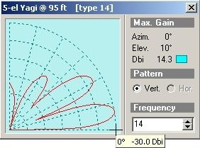
For example, see what happens to the curve of the 5-element yagi displayed below
left. At 0° the gain drops of 30 dB (- 30 dBi) ! In fact, in the field
practically no antenna develops a 0 dBi at those very low angles. The 5-element
Yagi displayed below shows its maximum gain (14.5 dBi) at 10° only (erected
close to 31m high or 95')...
|
|
|
Performance
of a 5-element Yagi calculated by Ham
CAP. |
The
left chart calculated for a 5-element Yagi with Ham
CAP, shows also very well that no sky wave or at least only the
weakest (-30 dBi) will leave your antenna at 0.1° of elevation. Using
this antenna model on the 20-m band, the value becomes positive (0 dBi)
from 1.2° of elevation only, and increases then rapidly to reach 14.3
dBi at 10° as displayed.
But
the VOACAP interface works does not request the same inputs parameters
as it works in a different way. If you must enter 3° (most of the time)
for the minimum takeoff angle, you must enter the maximum gain of the
main lobe as calculated by HFANT or another application like Ham CAP,
not the value at 3° of elevation. If you set the 14.3 dBi gain at 3°
for example your result will be wrong because at this elevation the gain
is usually close to -10 dBi, or 24 dB less. Such a difference mean that
your power ratio (signal strength) can fluctuate of a 200-factor if you
don't take care !
In other
words, if your takeoff angle and antenna gain are wrongly set, the
prediction will consider either that you use a 2 kW emitter or a
QRP station ! Here also, better to set the right values to expect accurate
forecasts, Hi !
Note
at last, that using an antenna showing a too narrow beam, say below 5-10° wide
only in either the vertical or horizontal plane (but very rare in amateur HF
installations), the Skyloc interferometer system can show that the signal at
receive location can display deep fading due to instantaneous variation in the
sky wave arrival angle. The QSB can reach 16 dB or more, the beam spreading up
to 8° on both side of the central angle per mode. This factor is not taken into
account by VOACAP that consider only single ray hops and predict a clustering of
angles arounf the median value or around several medians for multiple ray hop
modes. These lack of accuracy during the development of VOACAP affect the
prediction of signal strength as well.
Rx
Antenna
Contrarily
to the previous field, only one receive antenna can be
specified. But we have not to forget that VOACAP was
written for broadcast purposes first, where emitters usually work with several transmit antennas
tuned on specific frequencies to reach far countries in the best
conditions to avoid silent zones or signal losses.
In
most cases, if we believe the rule that states that "what is good for
receive is good for transmit", or "if you can hear him you can work
him", then the Rx ant = Tx ant. But to be accurate, like with the Tx
Antenna group, if the receive antenna is directional or displays a main lobe,
it is recommended to specify its bearing (e.g. the azimuth of the main lobe or
to select "at Tx"), the model, its gain, and its power gain expressed in
kW also.
Here
also, view from the transmitter, the antenna minimum takeoff angle (usually 3°)
is taken into account using only single ray hops what affects the prediction of
some errors in calculating the signal strength.
Like
the Tx Antenna field, the antenna gain is the value of the receive antenna main
lobe, not the value at 0.1 or 3° of elevation.
Clarification
Voilà,
that all folks, as should say a well-known animal ! Working top-down, this last
and 30th field achieves our settings and
ends the input process, at last ! ... Aaah ! (sigh).
As
you see there are a lot of information taken into account by VOACAP to establish
a forecast, and so much the better ! This is through all these parameters, added
to the list of ones ready to be displayed (see next page), that VOACAP and other
ICEPAC show all their power. No other amateur program (excepted those using the same
engine with or without additional functions)
provides such flexibility, synonymous obviously in this case, of complexity in taking into
account so many factors that might affect a transmission. Only VOACAP and alike
characterize the working conditions with so much details.
However,
I have never written that this flexibility and power were synonymous of
accuracy. This latter quality is related to algorithms used by the model, and
not to the amount of parameters used. In this regard, despite its numerous and
various input screens, VOACAP is perfectible as we explained earlier and will
tell again in the last page.
But
I feel that you have maybe an unresolved question that rises at the horizon :
with so many uncertainties and limitations associated to some fields, input
errors and other bias, you maybe wonder whether we don't have to give up your chance to
get an accurate prediction ? Not at all. You must know that VOACAP works
with median values and that you will get a prediction, which accuracy will
depend on values assigned to your input parameters. You will never get a result sure with 100%
confidence like "you have 100% reliability to reach this VY0 station S-9 with an S/N of 30 dB
at 1830 UTC with angles of arrival close to 10° in elevation during 5 minutes". Don't dream, no
application, even those running on supercomputers, can provide you such a solution...
To caricature I 'd say that for each of these answers you need a dedicated application.
In all other cases you will only get the big picture and a statistical answer.
Therefore you must very well know limitations and the meaning of each field before
to be able to interpret any result.
Now
that all inputs are complete and accepted by the system, let's see how to run propagation calculations and
display theses results.
Last
chapter
Forecasts
and outputs
|


