Introduction

The Sun is animated by a rotational motion which can be easily perceived currently, at the maximum of activity because the sunspots visible with naked eye* frequently appear. It is then possible to see these spots moving on the solar disc from East to West in some days. The precise observation of the spots - by means of a telescope and during some years - allows to notice that the rotation in the neighborhood of the equator of the Sun is faster than in the "high" latitudes (about ±40°). The statistical study of these observations shows that the rotation is 25,4 days at the equator and about 27 days at latitude ±40°. This difference of speed of rotation according to the latitude - called differential rotation - shows that the Sun does not behave like a solid body, at least on the surface. Sunspots are easily observable by projection and constitute tracers usually used by the amateurs. However, they present also inconveniences within the framework of the study of the differential rotation :

• They are closely related to areas with strong magnetic fields, often multipolar, called "active regions" and within which the field of speed of the material can be complex.
• Sun-spots are born, mostly evolve in group then disappear. During this development, the proper motion of spots in the group and the deformation or the dislocation of spots overlap the rotational component. The selection of the old isolated spots (type H/J in Waldmeier's classification), more stable but rarer, allows to reduce the component "proper motion" (Martres, 1999; Beck, 2000).
• The latitude of sun-spots varies between ±5° and ±40° during a solar cycle of activity. It turns out so impossible to make measures of the rotation beyond these values.

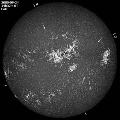
Is it possible, as an amateur, to observe this phenomenon by another way, without having observations of the sun-spots during a complete cycle ?

Methodology

The spectroscopy allows to measure the radial velocity vr of plasma by using the Doppler effect which results in a shifting of the wavelengths Δλ in the spectrum :

vr = c . Δλ / λ

At the equatorial limb of the Sun, the material moves about 2 km/s along the axis of aim. To apply this method to solar plasma requires to have the capacity to measure spectral shifts of some picomètres (10-12m). We leave there the possibilities of the amateurs... **

Let us return then to the method of the tracers. If we are able to observe the Sun, either in white light but in monochromatic light, i.e. in a very narrow spectral band (< 0,1nm), the observation of tracers others than the sunspots, distributed on a wide area on both sides of the equator, can open other horizons to us. So, the observation of the Sun using a monochromatic filter or a spectroheliograph in the line of the ionized Calcium (CaII: λ= 393,4 nm), makes appear structures little or not visible in white light. It is the case with faculae, chromospheric network, filaments, etc.... These structures are located in the chromosphere, at various altitudes ranging between few hundreds and few thousands km.

Among these elements which become thus accessible to the observation, brilliant points of the chromospheric network seemed to us to be able to serve as usefull tracers for the following reasons:

• These structures appear under the aspect of small brilliant spots from 5 to 10 " in diameter and, considering the weak resolution of the images (sampling with 2,5 " per pixel), seems almost punctual (Fig. 1, arrows). The pointing of the centre of these brilliant areas is rather easy and does not require calculation of barycenter.
• A first examination of the obtained images shows that these points of the chromospheric network have a sufficient lifespan so that one can follow their position during 1 or 2 days, sometimes more.
• Their distribution varies from the equator to more than ±60 ° in latitude, in any cases for this phase of the solar cycle.
• These objects are present outside the active regions, and we hope so that their proper movements are not going "to blur" too much the measure of the rotational motion. Their number should however allow to release the rotational component.

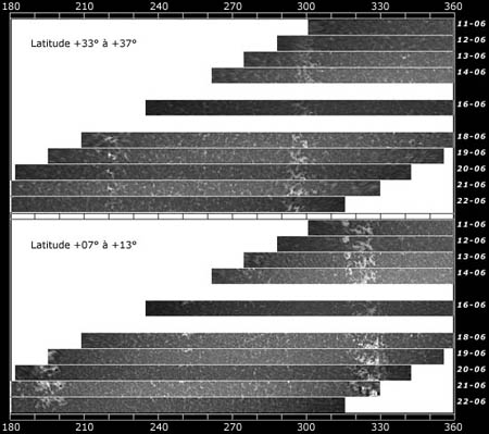
fig. 1 - The Chromospheric network, tracer of solar rotation

The choice of the tracer being made, it is now appropriate to examine the hard acquired images, i.e. to locate points of the network on images spaced in time, to measure their heliographic coordinates and to deduce the speeds of rotation from them. To facilitate at the same time their location and the measurement of their position, we appealed to the power of the data processing by realizing programs.

The purpose of a first software is to produce, from planisphere images ((cf. example), diagrams of evolution of a band parallel to the equator and some degrees wide in latitude. Such a shaping already reveals the differential rotation on the large faculae of the active regions (Fig. 2). So, we notice easily that their longitudinal drift is positive at latitude 10° while it seems sharply negative at latitude 35°.

fig. 2 - Revealing of the differential rotation

This synthetic representation allows especially a good visual location of the points of the network because the same region of the Sun is seen on various dates. Certain cases of identification are difficult and it is often necessary to refer to surrounding details to decide to associate or not two structures separated in time with the same point.

The second software allows to give concrete expression to this association by directly pointing by means of the mouse the same tracer on two nearby dates t1 and t2. The heliographic positions, dates as well as the other parameters are automatically stored in a spreadsheet. Every couple of positions allows to calculate then a speed of rotation :

ω = (l2 - l1) / (t2 - t1)

And the average latitude between the two dates :

φ = (φ1 + φ2) / 2

It is necessary to realize observations daily if possible to follow in best the movement of the points of the chromospheric network, which have a relatively short lifespan.

Data and results

The present results concerned the analysis of 73 daily images acquired with our spectroheliograph with CCD between April 22, 2000 and September 26, 2000. The coverage, globally 46 %, is not so very good. 20 diagrams were established in the interval of latitudes from -60° to +60°, with bands 6° wide. 1547 couples of positions were measured giving 1574 speeds.
These data were included in a graph with the heliographic latitude as X-coordinate and sidereal angular speed in degree per day as Y-coordinate(Fig. 3a). The examination of this graph shows that points are concentrated along a parabolic curve.

The relation between heliographic latitude φ and angular speed ω is usually expressed by the formulas :

ω(φ) = A + B sin²(φ)

or

ω(φ) = A + B sin²(φ) + C sin4(φ)

The first one describes rather well the rotation in the zone where one observes sunspots; the second reports better the rotation extended to the higher latitudes. The obtained values are indicated in the table 1. Given the very little weight of the parameter C, we will take into account only A and B. The number of measures is indicated in the column n.

Tableau 1 - Parameters of the model of sidereal rotation.

The dispersal of points is represented on the figure 3b. We saw previously (Rousselle, 2001) that the uncertainty of the measure of longitude was approximately 0,5 heliographic degree. The proper motions of the points of the chromospheric network also contribute to the dispersal of the values (Meunier, 1997).

The literature (Ward, 1966; Balthasar and Wöhl, 1980; Arévalo and al., 1982; Meunier, 1997) gives different values for the parameters A, B and C according to the various tracers, to the phase of the solar cycle, to the solar cycles, etc. … Comparison shows closer values A and B obtained here - rather high - to those corresponding in the young sunspots (type C and D) or to small structures associated with magnetic fields (Belvedere and al, on 1977), which is the case of the points of the network, and to a phase of maximum of sun activity (Balthasar and al., on 1986), which is also the case currently.

Let us note that there is a light asymmetry between the 2 hemispheres. This phenomenon is moreover observed as for the speeds of rotation as for the number of sun-spots (Wolf number) or as other indications of activity and can be much more marked.
The 2 models "north" and "South" are globally similar but the defect of a symmetry becomes more visible if one modifies the graph 3a by calculating the average speed of rotation inside bands of few degrees wide in latitude (Fig. 4). A width of 6° was chosen as compromise between the number of bands and the number of measures by band. weights are not equivalent.

Fig. 4 - Distribution of the speeds of rotation (curve) and distribution of the measures

The resultant graph, although strongly smoothed, presents undulations, notably in the north hemisphere, being able to result from different causes: speed of rotation was very differentiated in some bands, important proper motions, sub-sampling for some latitudes bands…

No significant correlation was revealing for the meridian movements. The precision of the measures is in that case much more determining.

Conclusion

It would seem so that one can reach - on the amateur level - approximate measurement of the solar differential rotation on a rather wide band of latitude in a duration of few months, the ideal being however to compare these results with a study concerning the same period and the same tracers. In addition, the increase of the number of measurementss and/or observers would allow to refine the results.

Bibliography

• Arévalo M.J., Gomez R., Vázquez M., Balthasar H., Wöhl H. : 1982, Differential Rotation and Meridional Motions of Sunspots from 1874 to 1902. Astron. Astrophys. 111, 266.
• Balthasar H., Vázquez M., Wöhl H. : 1986, Differential rotation of sunspots groups in the period from 1874 through 1976 and changes of the rotation velocity within the solar cycle. Astron. Astrophys. 155, 87.
• Balthasar H., Wöhl H. : 1980, Differential rotation and meridional motions of sunspots in the years 1940-1968. Astron. Astrophys. 92, 111.
• Beck J. : 2000, A comparison of differential rotation measurements. Solar Phys. 191, 47.
• Belvedere G., Godoli G., Motta S., Paternò L., Zappala A. : 1977, K faculae as tracers of the solar differential rotation. Ap. J. 214, 91.
• Martres M.J. : 1999, PMMPTS. L'Astronomie, 113, 85.
• Meunier N. : 1997, Diagnostic observationnels du champ magnétique solaire : distribution spatiale, dynamique et processus de génération. Thèse de doctorat d'Astrophysique et techniques spatiales. Université D. Diderot - Paris VII
• Rousselle P. : 2001. Spectrohéliographie à CCD… Et après? L'Astronomie, vol 115, 182.
• Ward F., : 1966, Determination of the solar rotation rate from the motion of identifiables features. Ap. J. 145,416.

Recommended book

• Beck R., Heinz H. , Reinsch K., Völker P. :1995, Solar Astronomy Handbook. Willmann-Bell, inc. Richmond, Virginia.

ooOoo

* II is reminded that, in the case of the Sun, the expression " naked eye " means "without magnifying device". A guaranteed quality protection filter is obviously necessary.

** See possibly the attempt mentioned in the page revealing of the sun rotation by spectroscopy