Spectroheliograph - solar differential rotation

Solar differential rotation

Introduction

In year 1611, Galileo systematically observes the sunspots and deduces solar rotation. Scheiner, profiting from 20 years of measurements, shows in 1630 that the spots close to the equator spend less time to cross the solar disc than the spots being to higher latitudes. It will be necessary to wait until 1863 for the establishment of the differential rotation law by Carrington. It also adopts a period of average solar sidereal rotation equal to 25.38 days and a frame of reference whose meridian line origin corresponds to the central meridian line on January 1st 1854, 12h UT.

Thus, a means of measuring solar rotation consists in recording the position of the sunspots on successive dates. One notes a movement from the East towards the West. this is called the tracers method (fig. 1).

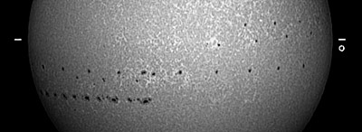
fig. 1 - description of solar rotation (01 to 06 August, 2003)

The use of a spectroheliograph (or a specific filter H-alpha or CaII) makes it possible to observe characteristic structures of chromosphere and inner corona : plages, chromospheric network, filaments, etc). Some of these structures are more frequent and cover a broader zone in latitude than sunspots. They thus are usefull to measure, quickly and from equator to high latitudes, the solar rotation.

Observing the Sun as often as possible, I wanted to see what it was possible to do about this for an amateur. Here is quickly exposed the method which I employ :

The images of the sun, are first of all corrected geometrically (more). Heliographic North, radius and center of the solar disc are measured.
The parameters P, Bo and Lo (respectively angle of position of the solar axis, heliographic latitude and heliographic longitude of the center of the solar disc) are interpolated from ephemerides.
Various methods are possible to measure the position of the tracers: either one superimpose a grid of co-ordinates (Stonyhurst) on the image and one reads the co-ordinates compared to the central meridian line directly (fig. 2), or one measures co-ordinates x and y of each tracer compared to the center and one calculates corresponding longitude and latitude with trigonometric formula (fig. 3), either one map the whole image on a rectangular co-ordinates frame. This last solution is very usefull for the following data-processing treatment (fig 4). The vertical white line indicates the position of the central meridian line at the moment of the observation. In practice, only the zone ranging between +/-60 degrees in latitude and +/- 80° in longitude compared to the central meridian line is mapped. The scale is 4 pixels per heliographic degree in both directions.

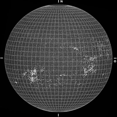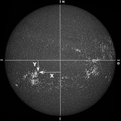
Fig. 2 - coordinates grid Fig. 3 - rectangular coordinates

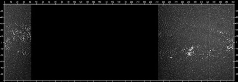
Fig. 4 - cylindrical projection ( august 05, 2003, CaII)

Every day, because of the solar rotation and of the revolution of the Earth around the Sun, the longitude of the central meridian (system of Carrington) decreases 13.2° approximately. It follows that the observed portion of Sun is gradually moved towards the left of the planisphere. This is illustrated by the figure 5 which shows 4 successive observations spaced out by 2 days (06 to 12 August , 2003, CaII).

By placing planispheres some above the others, the spots and the other characteristic elements seem arranged vertically and thus seem - at first sight - to be in a constant longitude.
It is now necessary to look carefully and to notice that, even with this breve scales of time and resolution, we can already detect changes of longitude for some spots. The small facula against the green line (August 06th) deviates from it slightly towards left the next days. An opposite movement appears for the facula situated to the right of the red line and near the equator. There are thus things which move on the surface of the Sun which go faster than the average near the equator and which slow down when we go towards the poles.
To make these movements more evident, it is necessary to use a large number of images in a larger scale but to stack so planispheres becomes fast badly convenient and ineffective.

Fig. 5 - planispheres sequence

Spots or other tracers having very small motions in latitude, we can cut bands of some degrees in latitude from every planisphere and stack them as previously. We so obtain a more compact document to be manipulated and which facilitates the visual detection of the longitudinal movements. The figure 6 resumes a band of 10° (-30° to -20°) and we notice easily the drift of the facule without the help of a vertical line.

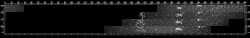
Fig. 6 - bands of 10° in lat. sequence

Concretely, the cylindrical projection is realized after each processing of spectroheliograms, i.e. after each observation, and for 3 wavelengths if possible (see archives). In year 2003 for example, I got 96 planispheres in the line of ionized calcium, over 6 months when I be able to observe (April to September). The division and stacking of the bands of latitude is automatically realized on all or only a selection of the annual observations by a specific program.
For the measure of the differential rotation I retained a height of 6° in latitude, what gives in finally 20 boards of 1500x5000 pixels, from 60 to 60° in latitude, to examine. Here is a small piece (fig. 7).

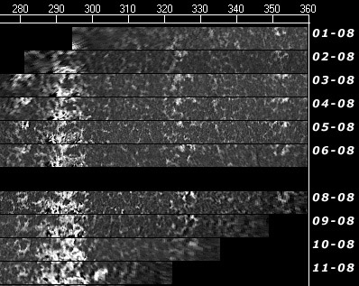
Fig. 7 - Sequence of 6° bands, centered on -15° in latitude, (100% scale)

I focused at the moment on brilliant points (5 to 10 ") of the chromospheric network, well visible in CaII, outside the active regions where appear groups of spots (more). They are plentiful near the equator but rather rare in the high latitudes and their life time seems to vary at least from 1 day (unusable) to 2 days, several times more. The location of points is visually made by taking into account the neighborhood to minimize errors. The speeds dispersion is rather high but the law of differential rotation is not so bal founded because of the large number of speeds measured.

This kind of studies, led by professionals, allowed - among other things - to show that the various tracers of rotation tend to have speed ranges which are appropriate for them, what would explain by a magnetic anchoring with various depthes under the photosphere.